

2.10.3 Unit Impulse FunctionOn occasion we confront a "continuous" random variable that has a positive probability of assuming one or more particular experimental values. It is difficult to extend the notion of probability density functions to cover this case, since for any finite fx(x) the probability of assuming an experimental value in the interval x to x +  x is approximately fx(x) x is approximately fx(x) x, becoming vanishingly small as x, becoming vanishingly small as  x x  0. 0.
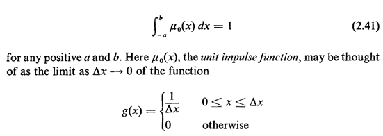
A mechanism for circumventing this problem is to define a function  0(x) that has area equal to 1
at x = 0. That is, 0(x) that has area equal to 1
at x = 0. That is,

Clearly, g(x) is a legitimate pdf since it is always nonnegative and it integrates to 1. Since any probabilistic statement involving pdf's must always involve integration, we need not concern ourselves with the "value" of  0(x) = 0(x) =  g(x) at x = 0 but only its integration properties
near x = 0. Since g(x) at x = 0 but only its integration properties
near x = 0. Since  0(x) has area 1 at
x = 0, the integral of any function h(x) multiplied by 0(x) has area 1 at
x = 0, the integral of any function h(x) multiplied by  0(x) is simply h(O), provided that the range of integration includes x = 0;
that is, 0(x) is simply h(O), provided that the range of integration includes x = 0;
that is,
for any positive a and b. For instance, a Bernoulli random variable having probability p of equaling 1 and (1 - p) of equaling zero may be summarized by the following probability "density" function: 
The cdf behaves as we wish; for instance, 
In a similar manner, we could write any pmf as a pdf using impulse functions. We could also use impulse functions to depict the pdf of a mixed random variable. |


