


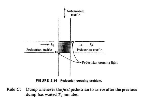
2.14 PEDESTRIAN CROSSING PROBLEMIn this section we study a problem involving the timing of a pedestrian street-crossing light. The problem provides a good illustration of many of the probabilistic modeling techniques that we have reviewed in this chapter, particularly the Poisson process. It also provides an example of applying mathematical modeling to the evaluation of technological alternatives in an urban setting. The problem is as follows. Pedestrians approach from the  side of the crossing in a Poisson manner with
average arrival rate side of the crossing in a Poisson manner with
average arrival rate  arrivals per minute (Figure 2.14). Each pedestrian then waits until a light is
flashed, at which time all waiting pedestrians must cross. We refer
to each time the light is flashed as a "dump" and assume that a dump
takes zero time (i.e., pedestrians cross instantly). Assume that the
left and right arrival processes are independent. arrivals per minute (Figure 2.14). Each pedestrian then waits until a light is
flashed, at which time all waiting pedestrians must cross. We refer
to each time the light is flashed as a "dump" and assume that a dump
takes zero time (i.e., pedestrians cross instantly). Assume that the
left and right arrival processes are independent.We wish to analyze three possible decision rules for operating the light:
Presumably, implementation of each rule requires a particular type of technology with its attendant costs, and thus it is important to determine the operating characteristics of each in order to understand tradeoffs between performance and cost. For each decision rule, determine:
We answer each part in sequence, analyzing each of the three decision rules as we proceed. 1. Let For interdump times fixed at T minutes, we simply require the expected
number of Poisson arrivals in an interval [0, T], which gives

If the decision rule is to dump whenever there are exactly N0 waiting
pedestrians, obviously the total number of pedestrians crossing will be
equal to N0 However, the probability that any particular one is a
left-to-right crossing pedestrian is

For rule C, the expected number of left-to-right crossing pedestrians during the pedestrian-initiated waiting period of duration T0 minutes is  LT0. However, we must also count the first arriving pedestrian who initiates
this waiting period; he has a probability equal to LT0. However, we must also count the first arriving pedestrian who initiates
this waiting period; he has a probability equal to  L/( L/( L + L +  R of being a "left-to-right" pedestrian. Thus, using a "left-pedestrian"
indicator random variable, added to a Poisson random variable, we obtain R of being a "left-to-right" pedestrian. Thus, using a "left-pedestrian"
indicator random variable, added to a Poisson random variable, we obtain

2. Let For decision rule A, 
For decision rule B, the probability that zero of the N0 crossing
pedestrians are left-to-right pedestrians is equal to the probability
that N0 successive independent Bernoulli trials yield a right-to-left
pedestrian. Thus,

For decision rule C, 
3. Let the three desired pdf's be fXA(.), fXB(.), and fXC(.),
respectively. Since we are finding the pdf's for the time between dumps
and since the decision rules utilize information on the total number of
arriving pedestrians (and rule A utilizes no information on arriving
pedestrians), we need only consider in this part the pooled Poisson
process having arrival rate The first pdf is simply the unit impulse located at T; thus,

The second pdf corresponds to the N0th-order interarrival time pdf for a
Poisson process with (pooled) arrival rate 
For the third pdf we use the fact that the time between dumps Xc can be
expressed as
But the time until the first pedestrian arrives is equal to the first-order interarrival time in a (pooled) process with rate  L + L +
 R, and this is simply a negative
exponential pdf with mean ( R, and this is simply a negative
exponential pdf with mean ( L + L +
 R)-1. Thus, the pdf for XC is simply the negative exponential
pdf shifted to the right by T0 minutes, R)-1. Thus, the pdf for XC is simply the negative exponential
pdf shifted to the right by T0 minutes,

4. Let For rule A, in which a dump occurs every T minutes, we can correctly
reason that his or her arrival time in the interval [0, T] is uniformly
distributed over the interval, and thus the waiting time until the end
of the interval is uniformly distributed, implying

To analyze rule B we must be a bit more careful. A randomly arriving
pedestrian is equally likely to be the first to arrive since the last
dump, the second to arrive, . . ., the N0th to arrive. Thus, the
probability that a randomly arriving pedestrian is the kth to arrive
since the last dump is equal to 1/N0 for k = 1, 2, . . . , N0. Given
that he or she is the kth to arrive, his or her conditional waiting time
until the next dump is distributed as an (N0 - k)order Erlang random
variable with parameter 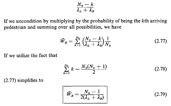
Does this make sense intuitively? To analyze rule C, let us condition on the total number of pedestrians
who arrive during the interval of length T0 initiated by the first
arriving pedestrian. Clearly, the first arriving pedestrian has an
expected wait of T0 minutes and any other arriving pedestrian prior to
the dump has an expected wait of T0/2 minutes. We seek to combine these two conditional expected waits in
an appropriate manner. Call ( 
To find now the expected unconditional waiting time,  ,
per pedestrian, we must multiply by the probability that a randomly
chosen pedestrian has crossed the street in a group of k + 1
pedestrians. This is a case of random incidence and the probability in
question [use the discrete analogue of (2.63)] is given by ,
per pedestrian, we must multiply by the probability that a randomly
chosen pedestrian has crossed the street in a group of k + 1
pedestrians. This is a case of random incidence and the probability in
question [use the discrete analogue of (2.63)] is given by
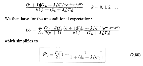
We can check the reasonableness of this result for two limiting cases: (1) as T0 becomes large compared to the mean passenger interarrival time (  L + L +
 R)-1,
the mean wait approaches one half the mean interdump time, a result in
agreement with (2.66) for the case in which the variance of the
interdump time is small compared to the square of the mean; and (2) as
T0 becomes very small, R)-1,
the mean wait approaches one half the mean interdump time, a result in
agreement with (2.66) for the case in which the variance of the
interdump time is small compared to the square of the mean; and (2) as
T0 becomes very small,
 approaches T, (which is also expected, since in that case nearly all
crossing pedestrians are first arriving pedestrians).
We could obtain (2.80) by another argument, based on "perturbation
random variables," as formalized in Section 3.8. Roughly, the argument
goes as follows. Each pedestrian must incur an average wait of T0/2
minutes. In addition, there is a certain probability that a randomly
arriving pedestrian must incur an additional mean wait of T0/2 minutes;
this probability is equal to the probability of being the first arriving
pedestrian. Thus, we could write

To compute the probability in the perturbation term, consider a very
long period of time during which N dumps, where N is a large number,
have taken place. This means that N "first pedestrians" have arrived and
an expected number of N( 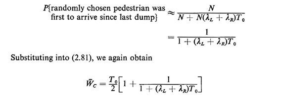
Note that the result above has been argued quite informally, in keeping with the informality of the perturbation argument. 5. This part is considerably easier than part 4. However, it is
instructive to compare the answers to those in part 4 for each of the
three decision rules. In part 4, the randomly arriving person is a
pedestrian and he or she thus "disturbs" the system. In this part the
randomly arriving person is strictly an observer, and thus he or she
does not affect the system. Call the times desired
All we need do to obtain the three required answers is apply (2.66)
derived for random incidence. Recalling that equation, in the context of
this problem, it states that the expected time until the next dump (from
the moment of the observer's arrival) is equal to one half the sum of
the mean squared and the variance of the interdump times, divided by the
mean. For instance, for decision rule A we have E[XA] = T and
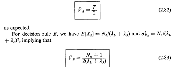
Note that this result is similar to that derived in part 4, except that the "+ 1" here is replaced by a "-1." Does this make sense intuitively? Can you derive (2.83) along the lines argued in part 4 to confirm this result? For decision rule C, we have 
This result, too, checks with our intuition in two limiting cases: as T0  0, 0,
  1/( 1/( L + L +
 R),
implying that the expected time until the next dump is equal to the
expected time of arrival of the next pedestrian. As T0 becomes large, R),
implying that the expected time until the next dump is equal to the
expected time of arrival of the next pedestrian. As T0 becomes large,
  [T0 +
( [T0 +
( L + L +
 R)-1]/2
which is one half the expected interdump
time; this result checks with (2.66) for the case in which the variance
of the
interdump time is negligibly small in comparison to the square of the
mean. R)-1]/2
which is one half the expected interdump
time; this result checks with (2.66) for the case in which the variance
of the
interdump time is negligibly small in comparison to the square of the
mean.
This completes our analysis of the pedestrian crossing problem. In addition to providing us with a good example of probabilistic modeling as applied to an urban service system, it has pointed to directions we wish to pursue in Chapters 3-5.
|


