|
 |
|
|
When a designer uses an interactive display to edit a circuit, that display is connected to the main computer via a frame buffer. A frame buffer is simply a section of memory that the computer fills with an image. Connected to the frame buffer is a display processor that converts the image memory into a video signal. There may also be a graphics accelerator under the control of the main computer for rapid manipulation of the frame-buffer memory. There are many different types of frame buffers, display processors, graphics accelerators, and displays. Most frame buffers are iconic, containing an equal amount of memory for each pixel, or point on the screen. These iconic frame buffers are merely arrays with no other structure.
Some frame buffers use complex display lists, which encode the image in a form similar to that of a computer instruction set. The amount of memory required to hold such an image varies with the complexity of the image, but it is usually less than would be required by an iconic frame buffer. Although using the display processor for display lists is more complicated and expensive, it allows the main computer to manipulate complex images more rapidly because less frame-buffer memory has to be modified to make a change.
Another distinction is whether the display is raster or calligraphic. Raster displays, which are the most common, have electron guns that sweep the entire surface of the screen in a fixed order. Calligraphic displays, sometimes called vector displays, are increasingly rare; they have electron guns that move randomly across the screen to draw whatever is requested. Needless to say, calligraphic displays never use iconic frame buffers but instead are driven from display lists. The calligraphic-display list processor is simpler than the raster-display processor, however, because it can usually send drawing instructions directly to the electron guns. When memory was expensive, this tradeoff of more complex display hardware for less memory made sense; today the most expensive component is the calligraphic display tube, so these are typically faked with display processors that drive iconic frame buffers connected to less expensive raster displays. A final problem with calligraphic displays is that they have difficulty filling a solid area on the screen, which makes them unpopular for IC design.
Once the type of display is understood, the quality must be determined. The three main factors in image quality are the availability of color, the number of pixels on the screen, and the number of bits for each pixel. A first and obvious choice is between black-and-white (sometimes called monochrome) and color displays. For IC design, color is very important because there are many layers that must be distinguished. Schematics designers have less of a need for color but can still use it to reduce the clutter of complex designs.
The next factor in display quality is its resolution in pixels per inch. The spatial resolution, the number of points on the screen, is usually lower for raster displays than for calligraphic displays. Raster displays typically have about 500 to 1000 pixels across and down. Less expensive displays, such as are found on personal computers, have half that number, and high-resolution displays, which are becoming more common, have twice that number. Calligraphic displays can typically position the electron gun at 4000 or more discrete points across the screen.
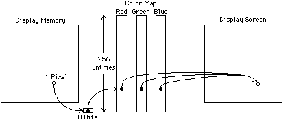
The number of bits available for each pixel determines the intensity resolution, which is just as important as the spatial resolution. Many black-and-white displays have only two intensity levels, on or off, making them bilevel displays. They can therefore store a complete pixel in one bit of memory. Simple color displays have eight colors determined by the bilevel combinations of red, green, and blue display guns. In order to have shading, however, more bits are needed to describe these three primary colors. For viewing by humans, no more than 8 to 10 bits of intensity are needed, which becomes 24 to 30 bits in color. Thus a high-resolution color display can consume over 3 megabytes of memory. For VLSI design, however, only 8 or 9 bits per pixel are needed; these can be evenly distributed among the color guns or mapped to a random selection. Color mapping translates the single value associated with a pixel into three color values for the display (see Fig. 9.1). In a typical map, 8 bits of pixel data address three tables, each 256 entries long. The individual entries can be 8 or more bits of intensity, allowing a full gamut of colors to be produced, provided no more than 256 different colors are displayed at any time.
 |
| FIGURE 9.1 Color mapping. One 9-bit pixel addresses a full color value in the map. |
Ideally, programming a frame buffer should be fairly simple, with the graphics accelerator doing all the difficult work of setting individual pixels. When such is the case, the controlling program needs to supply only vector endpoints, polygon vertices, and text strings to have these objects drawn. However, in less ideal situations, the CAD programmer may have to code these algorithms. The next section describes typical features of graphics accelerators and the following sections discuss the software issues.
There are a few operations that the frame buffer can typically do with or without a graphics accelerator. One feature that is often available is the ability to set the background color. On color-mapped displays, this simply means setting the map value for entry 0 of the table. On nonmapped displays, the entire surface must be filled with the desired background color and it must also be used whenever an object is erased.
One of the most useful features of many raster frame buffers is the write mask. This is a value that selects a subset of the bit-planes to use when changing the value of a pixel. For example, if the value 255 is written to a pixel in a 8-bit frame buffer and the write mask has the value 126, then only the top and bottom bits will be set and the others will be left as they were. Given this facility and a color map, one can assign a different bit-plane to each layer of a VLSI design and modify each plane independently of the others by masking them out (see Fig. 9.2). The drawing or erasing of layers takes place exclusively in the dedicated bit-plane without regard for the graphical interactions occurring with other layers in other bit-planes. With proper selection of color-map entries, each layer or bit-plane can be a different color and all combinations of layer overlap can be sensibly shaded.
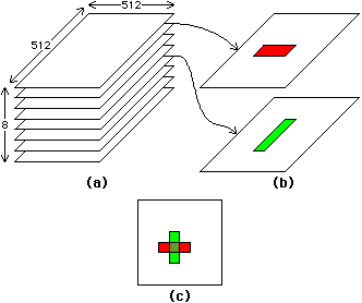 |
| FIGURE 9.2 Individual bit-plane control allows display memory to be organized by layer: (a) Display memory (b) The contents of two sample bit planes (c) The resulting display. |
For systems that have graphics accelerators, a number of hardware functions become available. One very common feature that is provided on raster displays is the ability to move a block of data on the screen quickly. This operation, called block transfer (or bitblt or BLT), is useful in many graphic applications. Block transfer can be used to fill areas of the screen and to move objects rapidly. Complex graphic operations can be done with the block transfer because it typically provides a general-purpose arithmetic and logical engine to manipulate the data during transfer. So, for example, an image can be moved smoothly across the display without obscuring the data behind it. This is done by XORing the image with the display contents at each change of location, and then XORing it again to erase it before advancing. The block-transfer operation is usually fast enough that it can be used to pan an image, shifting the entire screen in one direction and filling in from an undisplayed buffer elsewhere in memory. Such panning presumes that an overall iconic image, larger than what is displayed, is available somewhere else in memory. Of course, all this data moving is necessary only on raster displays, because display-list frame buffers can pan without the need for block transfer or large image memories.
Another feature possible with the block transfer operation is the rapid display of hierarchical structures. When the contents of a cell is drawn, the location of that cell's image on the screen can be saved so that, if another instance of that cell appears elsewhere, it can be copied. This display caching works correctly for those IC design environments in which all instances of a cell have the same contents and size. It suffers whenever a fill pattern is used on the interior of polygons because the phase of the pattern may not line up when shifted to another location and placed against a similar pattern. A solution to this problem is to draw an outline around each cell instance so that patterns terminate cleanly at the cell border [Newell and Fitzpatrick].
Of course, there are many special-purpose graphics accelerators in existence, due particularly to the advances in VLSI systems capabilities. Modern raster displays have accelerators that draw lines, curves, and polygons. Very advanced accelerators, beyond the scope of this chapter, handle three-dimensional objects with hidden-surface elimination. Control of these devices is no different than the software interface described in the following sections.
Lines to be drawn are always presented as a pair of endpoints, (x1, y1) and (x2, y2), which define a line segment on the display. A simple line-drawing algorithm divides the intervals [x1 x2] and [y1 y2] into equal parts and steps through them, placing pixels. This is problematical in many respects, including low speed and line-quality degradation. The problem of speed is that the interval and increment determination requires complicated mathematics such as division (especially painful when done in hardware). The line quality is also poor for such a technique because the choice of interval may cause bunching of pixels or gaps in the line. If the interval is chosen to be 1 pixel on the longest axis, then the line will be visually correct but still hard to compute.
The solution to drawing lines without complex arithmetic is to use
scaled-integer values for the determination of pixel increments.
The most popular technique also does all initial calculations in
terms of these scaled integers [Breshenham 65].
The algorithm makes use of an indicator that initially has the value
D = 2 ![]() y -
y - ![]() x
(where
x
(where ![]() y = y2 - y1
and
y = y2 - y1
and ![]() x = x2 - x1), and a current point
(x, y), which initially is
(x1, y1).
After plotting this point, x is incremented by 1, and y
increments by 1 only if D > 0.
If y increments, then D has the value
2(
x = x2 - x1), and a current point
(x, y), which initially is
(x1, y1).
After plotting this point, x is incremented by 1, and y
increments by 1 only if D > 0.
If y increments, then D has the value
2(![]() y -
y - ![]() x) added
to it; otherwise, it has the value 2
x) added
to it; otherwise, it has the value 2![]() y added to it.
This continues until (x, y) reaches
(x2, y2).
y added to it.
This continues until (x, y) reaches
(x2, y2).
The Breshenham algorithm is very fast because the terms can be precomputed and all of them require only addition and subtraction. The version described is, of course, for lines with a slope of less than one because x increments smoothly. For other lines, the coordinate terms are simply reversed.
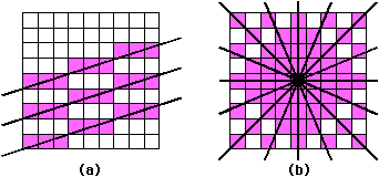
| Many CAD systems need textured lines to distinguish different objects. These can easily be drawn by storing a bit pattern that is rotated with the Breshenham counter, suppressing pixels that are not in the pattern. Thick lines can also be drawn by offsetting the startpoints and endpoints so that multiple parallel lines are drawn to fill in a region. However, unless these lines are very close together, there will be gaps left when the pixels of adjoining lines fail to fall on every position. This phenomenon is called a möire pattern and can occur wherever discrete approximations are made to geometry (see Fig. 9.3). Thus for very thick lines it is better to use a filled polygon. |
|
Polygons come in three styles: opened, closed, and filled. The first two are simply aggregates of lines but the third type is a separate problem in graphics. A filled polygon is trivially rendered if it is rectangular and has edges parallel to the axes. Since such polygons are common in VLSI design, special tests are worth making. Also, there have been some graphics accelerators that, when built into frame buffers, allow these rectangles to be drawn instantly. One system has a processor at each pixel that sets itself if its coordinate matches the broadcast polygon boundary [Locanthi]. Another system redesigns standard memory organization to allow parallel setting of rectangular areas [Whelan]. Rectangle filling is important because it is a basic operation that can be used to speed up line drawing, complex polygon filling, and more.
The problem of filling arbitrary polygons is somewhat more difficult. As with line drawing, there are many methods that produce varying quality results. One method is the parity-scan technique that sweeps the bounding area of the polygon, looking for edge pixels. The premise of this algorithm is that each edge pixel reverses the state of being inside or outside the polygon. Once inside, the scanner fills all pixels until it reaches the other edge. There is an obvious problem with this method: Quantization of edges into pixels may leave an incorrect number of pixels set on an edge, causing the parity to get reversed. Attempting to use the original line definitions will only make the mathematics more complex, and there may still be vertices of one point that confuse the parity. A variant on this technique, called edge flag [Ackland and Weste], uses a temporary frame buffer and complements the pixels immediately to the right of the polygon edges. This method works correctly because double complementing, which occurs at vertices, clears the edge bit and prevents runaway parity filling. When all edges have been entered into the temporary frame buffer, parity scan can be used to fill the polygon correctly.
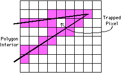
| Another polygon-fill method that has problems is seed fill. Here, a pixel on the interior is grown in a recursive manner until it reaches the edges. As each pixel is examined, it is filled, and any neighboring pixels that have not been filled are queued for subsequent examination. This method can use large amounts of memory in stacking pixels to be filled and it also may miss tight corners (see Fig. 9.4). Additionally, there is the problem of finding an interior point, which is far more complex than simply choosing the center. To be sure that a point is inside a polygon, a line constructed between it and the outside must intersect the polygon edges an odd number of times. This requires a nontrivial amount of computation because the process is expensive and still does not suggest a way of finding an interior point, only of checking it. Techniques for finding the point include (1) starting at the center, (2) advancing toward vertices, and (3) scanning every point in the bounding rectangle of the polygon. |
|
The best polygon-fill algorithm is dependent on the available hardware. If special-purpose hardware can be constructed, polygons can be filled almost instantly. For example, there is a hardware frame buffer that does a parallel set of all pixels on one side of a line [Fuchs et al.]. This can be used to fill convex polygons by logically combining interior state from each polygon edge.
|
The hardware for setting pixels on one side of a line must compute
the equation:
Ax + By + C = 0 |
|
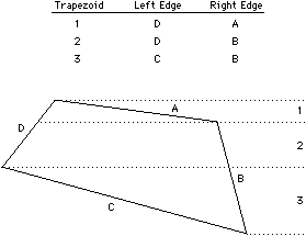
| When there is no fancy hardware for edge filling, an alternative is to analyze the polygon and to reduce it to a simpler object. For example, convex polygons can be decomposed into trapezoids by slicing them at the vertices. The result is a left- and right-edge list that, when scanned from top to bottom, gives starting and ending coordinates to be filled on a horizontal line (see Fig. 9.6). At each horizontal scan line there is only one active edge on each side and these edges can be traversed with Breshenham line drawing. Pixels between the edges can be filled with size n × 1 rectangle operations. |
|
Nonconvex polygons must first be decomposed into simpler ones. This requires the addition of cutting lines at points of inflection so that the polygon breaks into multiple simpler parts. Alternatively, it can be done using the trapezoid method described previously with a little extra bookkeeping for multiple fill pieces on each scan line [Newell and Sequin].
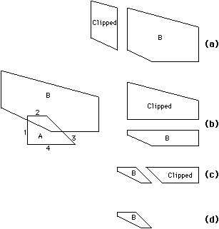
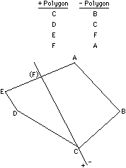
Clipping is the process of removing unwanted graphics. It is used in many tasks, including complex polygon decomposition, display-window bounding, and construction of nonredundant database geometry. Two clipping algorithms will be discussed here: polygon clipping and screen clipping.
| In polygon clipping, the basic operation is to slice an arbitrary polygon with a line and to produce two new polygons on either side of that line. Figure 9.7 shows how this operation can be used to determine the intersection of two polygons. Each line of polygon A is used to clip polygon B, throwing out that portion on the outside of the line. When all lines of polygon A have finished, the remaining piece of polygon B is the intersection area. |
|
The polygon-clipping algorithm to be discussed here runs through the points on the polygon and tests them against the equation of the clipping line [Catmull]. As mentioned before, a line equation is of the form:
The clipper takes each point in the polygon and uses the equation to place
it in one of two output lists that define the
two new split polygons.
Three rules determine what will happen to points from the original
polygon as they are sequentially transformed into the two clipped polygons.
These rules use information about the current point and the previous
point in the original polygon (see Fig. 9.8):
|
|
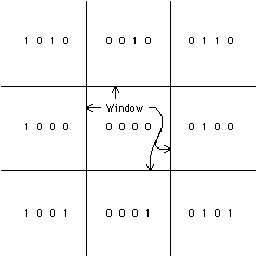
| There are other clipping methods that apply to different needs, the most common being screen clipping. In screen clipping, vectors must be clipped to a rectangular window so that they do not run off the edge of the display area. Although this can be achieved with four passes of polygon clipping, there is a much cheaper way to go. The Sutherland-Cohen clipping algorithm [Newman and Sproull] starts by dividing space into nine pieces according to the sides of the window boundaries (see Fig. 9.9). A 4-bit code exists in each piece and has a 1 bit set for each of the four window boundaries that have been crossed. The central piece, with the code 0000, is the actual display area to which lines are clipped. Computing the code value for each line endpoint is trivial and the line is clearly visible if both ends have the code 0000. Other lines are clearly invisible if the bits of their two endpoints are nonzero when ANDed together. Lines that are not immediately classified by their endpoint codes require a simple division to push an endpoint to one edge of the window. This may have to be done twice to get the vector completely within the display window. |
|
Display of text is quite simple but can be complicated by many options such as scale, orientation, and readable placement. The basic operation copies a predesigned image of a letter to the display. Each collection of these letters is a typeface, or font, and there may be many fonts available in different styles, sizes, and orientations. Although these variations of the letter form may be simple parameters to algorithms that can be used to construct the font [Knuth], it is easier and much faster to have fonts precomputed.
When placing text on top of drawings it is important to ensure the readability of the letters. If it is possible to display the text in a different color than the background drawing, legibility is greatly enhanced. An alternative to changing the text color is to use drop shadows, which are black borders around the text (actually only on the bottom and right sides) that distinguish the letters in busy backgrounds. A more severe distinction method is to erase a rectangle of background before writing the text. This can also be achieved by copying the entire letter array instead of just those pixels that compose the letter.
Of course, proper placement of text gives best results. For example, when text is attached to an object, it is more readable if the letters begin near the object and proceed away. Text for lines should be placed above or below the line. Excessive text should be truncated or scaled down so that it does not interfere with other text. Text becomes excessive when its size is greater than the object to which it attaches. All text should be optional and, in fact, the display system should allow any parts of the image to be switched on and off for clutter reduction. As anyone who has ever looked at a map can attest, text placement is a difficult task that can consume vast resources in a vain attempt to attain perfection. A CAD system should not attempt to solve this problem by itself, but should instead provide enough placement options that the user can make the display readable.
There are many curved symbols that need to be drawn on the screen.
The simplest is the circle, which can be drawn with the same method
as a line: Breshenham's algorithm [Breshenham 77].
The technique is to draw only one octant (the upper-right, from twelve
o'clock to one-thirty) and mirror it eight times to produce a circle.
For the purpose of algorithm description, the circle is centered
at (0, 0) so that
for a radius R the octant that is drawn is from (0, R) to
(R / ![]() 2,
R /
2,
R / ![]() 2).
For each point (x, y) in this octant, the seven other points
(-x, y), (x, -y), (-x, -y),
(y, x), (-y, x), (y, -x),
and (-y, -x) are also drawn.
2).
For each point (x, y) in this octant, the seven other points
(-x, y), (x, -y), (-x, -y),
(y, x), (-y, x), (y, -x),
and (-y, -x) are also drawn.
The Breshenham method proceeds as follows:
Initially start at
x = 0, y = R, and D = 3 - 2R.
At each step, increment x and conditionally decrement y if
D![]() 0.
When y is decremented, add 4(x - y)+10 to D
and when y is not decremented, add 4x+6 to D.
Proceed until x
0.
When y is decremented, add 4(x - y)+10 to D
and when y is not decremented, add 4x+6 to D.
Proceed until x ![]() y at which point the octant
is drawn.
y at which point the octant
is drawn.
Filled circles work the same way except that for each pair of octants at the same horizontal level, an n × 1 rectangle is drawn between the points. Thus for point (x, y) on the octant, fill from (-x, y) to (x, y), from (-x, -y) to (x, -y), from (-y, x) to (y, x), and from (-y, -x) to (y, -x).
Arcs of circles are difficult to draw because they can start or end anywhere. For the Breshenham method to be used, the number of full and partial octants must be determined and carefully tracked to know where to draw. Also, the Breshenham code must be able to end in mid-octant or to run backwards as needed by the arc. Arcs can be better drawn if they are first converted to vectors. There are many published sets of algorithms for vector approximation of curved shapes [Rogers and Adams].
Noncircular curves can be drawn in any number of ways, but the most common technique is the spline. The spline is a smooth curve that follows a set of control points. Unlike other curve methods, the spline can handle any number of points and produce a curve that is continuous in both the first and second derivatives. The disadvantage of the spline is that the curve does not necessarily pass through the control points, only near them. Other curve methods such as Hermite and Bezier [Bezier] have the opposite properties: They do pass through the control points but do not extend as cleanly to large numbers of points.
The B-spline (not to be confused with the Beta-spline [Barsky and Beatty]) is defined by two functions: X(t) and Y(t). As the value of t goes from 0 to 1, these functions describe the curve. It is necessary to break the control points into groups of four where each group defines a different equation for X(t) and Y(t). After the curve for points 1,2,3,4 is drawn, the points are advanced by one and the curve for points 2,3,4,5 is drawn. This continues until points n - 3, n - 2, n - 1, n are drawn at which time the entire spline has been rendered.
Formally, X(t) = T M Gx and
Y(t) = T M Gy
where T, M, Gx, and
Gy are matrices.
The matrix T is a simple shorthand for quadratic expansion:
|
|
| M | = | 1/6 | x | -1 | 3 | -3 | 1 |
3 | -6 | 3 | 0 | ||||
-3 | 0 | 3 | 0 | ||||
1 | 4 | 1 | 0 |
Putting these matrices together produces the following functions:
| X(t) | = | Xi(-t3+3t2-3t+1) + Xi+1(3t3-6t2+4) + Xi+2(-3t3+3t2+3t+1) + Xi+3t3 |
| Y(t) | = | Yi(-t3+3t2-3t+1) + Yi+1(3t3-6t2+4) + Yi+2(-3t3+3t2+3t+1) + Yi+3t3 |
Frame buffer programming can be a bottomless pit of effort because the user is never satisfied and always wants more. However, there is a standard tradeoff of speed and functionality that must be balanced, and the CAD system with too many cute display options may begin to be too slow for comfort. Users become accustomed to anything in time, so the display should do its best and leave it there.
Transformations are used to modify coordinates prior to rendering them, so that the figures change position, size, or orientation. Although some displays have built-in transformation facilities, programmers may have to do these operations explicitly. Position transformations are trivially implemented with addition, and scale transformations simply require multiplication. The only difficult transformation is rotation.
To rotate a point (x, y) by ![]() degrees about the origin, compute
the point:
degrees about the origin, compute
the point:
|
Previous |  |
Table of Contents | Next | |
Static Free Software |  |