


2.10 PROBABILITY DENSITY FUNCTIONSMany random variables encountered in practice are distributed over a continuous rather than a discrete set of values. Examples include the time one waits at a bus stop until the next bus arrives, the tons of trash collected in a city on a given day, the distance a social worker in the field will travel on a given day, and the amount of electricity consumed by a household during a year. Just as probability mass functions (pmf's) allowed us to explore the probabilistic behavior of discrete random variables, probability density functions (pdf's) allow us to do the same for continuously distributed random variables. We define a pdf for the (continuous) random variable X as follows: fx(x) dx  probability that the random variable X assumes an
experimental value between x and x + dx on a performance of the experiment probability that the random variable X assumes an
experimental value between x and x + dx on a performance of the experimentNote that our definition is not stated in terms of the probability that random variable X assumes exactly the value x; for a purely continuous random variable, this probability is zero. Thus, in order to make any probability statement using pdf's, one must integrate the pdf (even if only over an infinitesimal interval of length dx). Some random variables occurring in practice are mixed; that is, they have a purely continuous part and they have a discrete part, An example could be the location of a bus at a random time along a straight-line street route; the bus might be viewed as uniformly distributed over the route except for a probability pi of being located at X = xi, the location of the ith stop (i = 1, 2, . . . , N). In this case  is the "probability that the random
variable X is discrete" and (1 - ) is the
probability that it is continuous. To analyze the probabilistic behavior of X, we would treat
separately each of the two components of X (discrete and continuous),
and then combine the results using methods of conditional probability
(see Problem 2.2). Thus, whenever possible throughout the remainder of
this book, a continuous random variable is viewed as a purely continuous
(rather than mixed) random variable. Still, on occasion it is necessary
to consider a "continuous" random variable that has a positive
probability of assuming a particular value. We do this with the
unit impulse function, as shown later in this section. is the "probability that the random
variable X is discrete" and (1 - ) is the
probability that it is continuous. To analyze the probabilistic behavior of X, we would treat
separately each of the two components of X (discrete and continuous),
and then combine the results using methods of conditional probability
(see Problem 2.2). Thus, whenever possible throughout the remainder of
this book, a continuous random variable is viewed as a purely continuous
(rather than mixed) random variable. Still, on occasion it is necessary
to consider a "continuous" random variable that has a positive
probability of assuming a particular value. We do this with the
unit impulse function, as shown later in this section.Since probabilities must be nonnegative, we must have fx(x)  0. But
unlike the pmf, whose value cannot exceed unity, there is no upper bound
on the value of a pdf. A fundamental probabilistic statement involving a
pdf relates the pdf to its cumulative distribution function (cdf), 0. But
unlike the pmf, whose value cannot exceed unity, there is no upper bound
on the value of a pdf. A fundamental probabilistic statement involving a
pdf relates the pdf to its cumulative distribution function (cdf),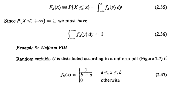
The cdf grows linearly from zero at U = a to 1 at U = b (Figure 2.8). The uniformly distributed random variable is often implied when the term "random" is used in problem statements, although we will attempt to avoid such ambiguous terminology here. 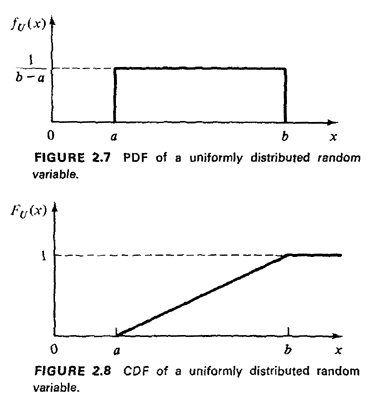
The compound pdf allows us to study two or more continuous random variables simultaneously. For two random variables X and Y, their compound pdf is given by 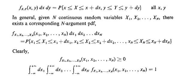
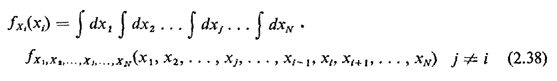
In cases involving multiple random variables, X1, X2, . . . ,XN, one may still be interested in the marginal pdf for Xi,fxi(xi), defined so that fxi(xi)dxi P{xi  Xi
xi + dxi}. We can
calculate the marginal from the joint pdf simply by integrating over
all the other random variables. Xi
xi + dxi}. We can
calculate the marginal from the joint pdf simply by integrating over
all the other random variables.
|