3.1 FUNCTIONS OF RANDOM VARIABLES:
DERIVED DISTRIBUTIONS
Often when examining a system we know by hypothesis or
measurement the probability law of one or more random
variables, and wish to obtain the probability laws of other
random variables that can be expressed in terms of the
original random variables. The random variables in the second set
are functions of the random variables in the first
set. We call this a problem of derived distributions, since we
must derive the joint probability distribution(s) for the
random variables in the second set. Derived distribution problems
can arise with discrete, continuous, or mixed
random variables.
There are many special techniques for deriving distributions, but
we will focus on a "never-fail" method.
Virtually all of the work associated with this method occurs in
the joint sample space of the original random
variables; the never-fail method is simply a systematic procedure
for carrying out Step 4 ("working in the sample
space") in a probabilistic modeling analysis.
Suppose that the original set of random variables is given by
{X1, X2, ..., XN} with joint cdf
FX1, X2,...,XN(·).
Suppose that there are M random variables
Y1, Y2, ..., YM, each of which can be
expressed as a function of X1, X2, ..., XN,
namely Yi = gi(X1, X2, ...,
XN), i = 1, 2, ..., M. Then the never-fail method, called the
cumulative distribution method, allows computation of the joint
cumulative distribution function for the Yi's,

as follows:
a. Identify the set of points in the original
(X1, X2, ..., XN) sample space that
corresponds to the joint event

b. For each set of values for the y1's, [y1, y2, . . . , yM],
determine by summation or integration the probability in the
(X1, X2,... XM,) sample space of this joint event, thereby obtaining
FY1,Y2... Ym(y1,y2,...yM) -  < y1,y2,...yM < +
If the random variables are continuous, we can find the joint pdf
for {Y1, Y2,... YM} by taking partial derivatives of
FY1,Y2,...YM (·) with respect to each of its arguments,

If they are discrete, the pmf is found simply by using the cdf
and subtracting appropriate successive values.
While the method described in its full generality may appear
intimidating, applying it carefully in a step-by-step
manner makes problems much easier to solve. Fortunately, for many
problems of interest the number of variables
involved i s small, often with neither M nor N exceeding 2.
Gaining proficiency in this aspect of probabilistic
modeling seems to require study of numerous examples, to uncover
potential pitfalls that await the unwary analyst.
Thus, we will analyze many examples, most of which are of
independent interest in the analysis of urban service
systems. Continuous random variables appear to give the greatest
difficulty to those first learning use of the
method, and thus our focus will be on continuous random
variables. Examples involving discrete random variables
are given in the problems. (See Problem 3.2 for strictly discrete
random variables and Problems 3.24 and 3.30 for
"mixed" random variables.)
Example 1: Response Distance of an Ambulette
This first example will provide a framework for demonstrating
several characteristics of "derived distribution" problems.
Suppose that a public safety vehicle travels back and forth along
a straight highway, the traveling perhaps to find
motorists in need of assistance. Also, along this highway
accidents can occur that create a need for on-scene assistance by
the vehicle. The vehicle is dispatched by radio to these
accidents. Because of its limited on-board emergency medical
equipment, we call the vehicle an ambulette. We are interested in
determining the probability law of the travel distance for
the ambulette to reach a random medical emergency.
Solution
Following the general discussion above, a derived distribution
problem is like any other probabilistic modeling problem;
it requires that we do four things to model the experiment:
| STEP 1: | Define the random variables of interest.
| | STEP 2: | Identify the joint sample space.
| | STEP3: | Determine the joint probability distribution over the sample space.
| | STEP 4: | Work within the sample space to determine the answers to any
questions about the experiment.
|
As discussed above, the activity specific to derived distributions (functions of
random variables) occurs in Step 4.
1. Random variables. Suppose that the highway is of unit length. Then the two key
random variables would be
X1 = location of the medical emergency, 0  X1 X1  I
I
X2 = location of the ambulette at the moment of dispatch, 0  X2 X2
Later, when we are interested in travel distance, assuming U-turns are possible and
permissible everywhere, the travel
distance D can be expressed as a function of X1 and X2, D = |X1 - X2|
2. Joint sample space. The joint sample space is the unit square in the positive
quadrant (0  X1 X1 1, 0
1, 0  X2 X2  1). 1).
3. Joint probability distribution. We will assume that the locations of the ambulette
and the medical emergency
are uniformly, independently distributed over the highway. In practice, the three
assumptions entailed in such a statement
would have to be argued for plausibility and measurements might have to be taken.
Naturally, the analysis could also
proceed with an alternative set of assumptions. Since we are now dealing with strictly
continuous random variables, we will
work with the joint probability density function, which is

4. Work in the sample space. This is the point at which the never-fail method for
deriving distributions comes
into play. We want the probability law of

Here, in our general notation, N = 2 and M = 1 and we are confronted with what is
sometimes called a 2-to-1 transformation.
To apply the never-fail method for finding the cdf of D, FD(y), we first locate the
region in the (XI, X2) sample space
corresponding to the event (D < y). Formally, the steps are written as follows:

To remove the absolute value operator, we consider two cases
separately: case 1: X1  X2; case 2: X1 < X2
. For the first case,
D = X1 - X2 and experimental values x1 and x2
of X1 and X2,
respectively, must lie between the line x2 = x1 and x2
= xI - y
(Figure
3.1). For the second case, D = X2 - X1, and experimental values
of X1 and X2 must lie between the line x2 = x1
and x2 = xI + y.
Consideration of these two cases gives rise to the shaded region
in the sample space in Figure 3.1. Once we have
determined such a region, we have identified the set of points
corresponding to the event of interest: [D < y), thereby
completing step a of the never-fail method. This is often the
most difficult part of a derived distribution problem. Note that
determination of this region in no way depended on the joint pdf
for X1 and X2; thus, the "work" invested to this point could
be applied to several alternative models, each with its own joint
pdf for X1 and X2. X2; case 2: X1 < X2
. For the first case,
D = X1 - X2 and experimental values x1 and x2
of X1 and X2,
respectively, must lie between the line x2 = x1 and x2
= xI - y
(Figure
3.1). For the second case, D = X2 - X1, and experimental values
of X1 and X2 must lie between the line x2 = x1
and x2 = xI + y.
Consideration of these two cases gives rise to the shaded region
in the sample space in Figure 3.1. Once we have
determined such a region, we have identified the set of points
corresponding to the event of interest: [D < y), thereby
completing step a of the never-fail method. This is often the
most difficult part of a derived distribution problem. Note that
determination of this region in no way depended on the joint pdf
for X1 and X2; thus, the "work" invested to this point could
be applied to several alternative models, each with its own joint
pdf for X1 and X2.
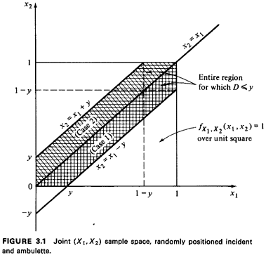
Step b of the never-fail method requires that we integrate
fx1,x2,(·) over the set of points in the shaded region to obtain
FD(y). Since the joint X1, X2 pdf is uniform over the unit
square, we can perform the integration by computing areas in the
sample space. (Conceptually, each area is multiplied by "l," the
height of the pdf at that point, to yield a probability
measured as a volume.) By computing areas of the triangles not in
the shaded region,

we have now completed step b of the never-fail method and we are
"done." [What do we know about FD(-2) or FD ?] ?]
Should we desire the pdf of D, we differentiate, obtaining

From the pdf (or cdf) we can determine anything that is desired
concerning
D. For instance, the expected value (or mean value) of D is

These results will be of use in our further work.
A system administrator may be interested in knowing the effects
on travel distance of prepositioning the ambulette at
the center of the interval depicting the highway, thus fixing X2
Then the joint sample space is the straight line indicated in
Figure 3.2. If the new travel distance is D'=|X1-1/2|, the
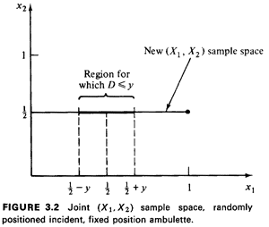
region for which (D'  y) is the line segment of length 2y
centered at X1=1/2. Integrating the (uniform) pdf of X1, we have
FD'(y) =P{D' y) is the line segment of length 2y
centered at X1=1/2. Integrating the (uniform) pdf of X1, we have
FD'(y) =P{D'  y)=
P{ | X - 1/2 | y)=
P{ | X - 1/2 |  y)= 2y (O y)= 2y (O  y y
 1/2). Thus, the pdf of D'is 1/2). Thus, the pdf of D'is

How could this result also be obtained by inspection? The mean
and variance are

Thus, a change in deployment policy resulting in an ambulette
prepositioned at the center of its service area rather
than randomly patrolling its service area reduces mean travel
distance by 25 percent, the variance of the travel
distance by 62.5 percent, and, perhaps important in "worst-case"
analyses, the maximum possible travel distance by
50 percent.
Question: How would one determine (or estimate) the joint
distribution function for X1 and X2 in practice?
Further work: Problems 3.2-3.4.
Extension: Scaling
We often select the scale of a probabilistic modeling problem for
analytical convenience. For instance, if the
length of highway analyzed in Example I had been 13.72
kilometers, the factor of 13.72 would have occurred in
numerous places (making the analysis obviously less attractive).
Thus, after performing the analysis for a
conveniently scaled problem, we often rescale it to suit the
real-world situation at hand. Scaling can also occur when
switching systems of measurement, say from British units to
metric units.
Suppose that we have derived the probability law for W, given one
scale, and we wish to find the moments and
the probability law of
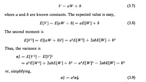
In words, multiplying a random variable by a constant results in
its variance being multiplied by the square of that
constant.
We can also derive the probability law of V (assumed to be
continuous) using the never-fail method. The
analysis proceeds as follows:

To proceed further, we must distinguish two cases: case 1: a>0; case2;a<0.

These equations constitute the answer to our problem. For
instance, in the ambulette example, if a = 13.72
kilometers and b = 71.09 kilometers, we would be modeling a
13.72-kilometer stretch of highway starting 71.09
kilometers from the origin. Returning to the patrolling ambulette
example, the cdf for X1 becomes
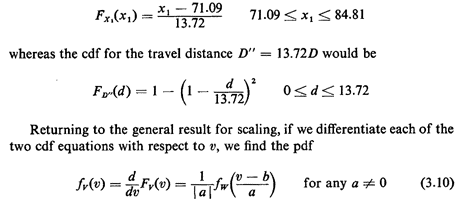
You might find it helpful to sketch several different
applications of this result.
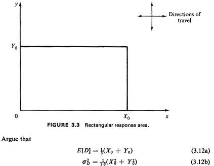
Exercise 3.1: Rectangular Response Area Suppose that we have an
X0-byY0 rectangular response area for the
ambulette (Figure 3.3), with sides of the rectangle parallel to
the coordinate axes. The location of the medical
emergency (X1, Y1) and of the ambulette (X2, Y2) are
independently uniformly distributed over the response area.
Travel distance occurs according to the "right-angle" metric,
D=|X1 -X2| + |Y1 - Y2| (3.11)
Example 1: Revisited (Min and Max)
Suppose we are interested in the coordinates that determine a
dispatch incident, X1 and X2, without regard to which location
represents the ambulette and which the medical emergency.
Instead, we may be concerned with the rightmost coordinate R
and the leftmost coordinate L. For instance all points between R
and L may be exposed to siren and lights as the ambulette
passes at high speed. Thus, the joint probability law of R and L
would be of interest. We will ignore scaling and assume
that all locations, as before, occur in the interval [0, 1].
Solution
Since we have already performed Steps 1-3 in describing the
experiment, we are ready to go to Step 4 (work in the sample
space) and employ the neverfail method. The random variables that
are functions of the original random variables are

We wish to derive the joint probability law for R and L. This is
sometimes called an N = 2-to-M = 2 transformation. To
execute step a of the never fail method, we proceed formally as follows:

To proceed from here, we consider separately each of the two events
in braces and "merge" these later by intersection.That is, we can write

To determine the set of points in the (X1, X2) rample space
corresponding to Max (X1, X2)  r, we again consider two
cases: case 1: X1 r, we again consider two
cases: case 1: X1  X2; case 2: X1 X2; case 2: X1
 X2. For case 1, Max (X1,
X2) = X1 and the event Max (X1, X2) X2. For case 1, Max (X1,
X2) = X1 and the event Max (X1, X2) r corresponds to
the set of points to the left of the line x1 = r (Figure 3.4).
Similarly, for case 2, Max (X1, X2) = X2 and the event Max (X1,
X2)
  r corresponds to the set of points below the line X2 =
r. Combining these two cases, the event Max (X1, X2) r corresponds to the set of points below the line X2 =
r. Combining these two cases, the event Max (X1, X2)  r
corresponds to the square of area r2 shown in Figure 3.4. r
corresponds to the square of area r2 shown in Figure 3.4.
Proceeding in a similar manner for Min (X1, X2)  1, we again
consider case 1: X1 1, we again
consider case 1: X1  X2, and case 2: X1 X2, and case 2: X1  X2. For
case 1, Min (X1, X2) = X2 and the event Min
(X1, X2)
  1
corresponds to the set of points below the line x2 = 1 (Figure
3.4). For case 2, Min (X1, X2) = X1 and the event Min (X1, X2) 1
corresponds to the set of points below the line x2 = 1 (Figure
3.4). For case 2, Min (X1, X2) = X1 and the event Min (X1, X2)
 1 corresponds to the set of points to the left of the line x1
= 1. Combining these two cases, the event Min (X1, X2) 1 corresponds to the set of points to the left of the line x1
= 1. Combining these two cases, the event Min (X1, X2)  1
corresponds to the L-shaped region shown in Figure 3.4. 1
corresponds to the L-shaped region shown in Figure 3.4.
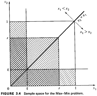
The intersection of the two events found above yields the event
of interest, {R  r, L r, L
 l}, shown in the crosshatched
region in Figure 3.4. We have now completed step a of the
never-fail method, l}, shown in the crosshatched
region in Figure 3.4. We have now completed step a of the
never-fail method,
To carry out step b all we need to do is to integrate the joint
pdf fx1, x2(·) over the region (event) found in Step 1. Again,
because of the special nature of this sample space and its
probability assignment, we can do this by working directly with
areas in the sample space. By computing the relevant areas, we
obtain

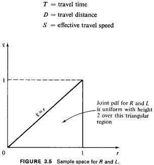
The joint R, L sample space is shown in Figure 3.5. The joint pdf
of R, L over this triangular region is uniform. Does this
make sense intuitively?
Example 2: Travel Time
Suppose that it is not travel distance we are interested in but
rather travel time. If we define random variables
time is related to distance and speed by the familiar equation

Solution
In general, to obtain the pdf of T we would require the joint pdf
of D and S, say fD, S(x, s). The never-fail method would
proceed as follows:

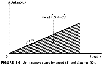
The event corresponding to [D  tS) in the (D, S) sample space is
shown in Figure 3.6. In principle, all we need do is
integrate the joint D, S pdf over this region for each value of t
to obtain the cdf for T, FT(t). 1 tS) in the (D, S) sample space is
shown in Figure 3.6. In principle, all we need do is
integrate the joint D, S pdf over this region for each value of t
to obtain the cdf for T, FT(t). 1
As a simple example, suppose that the speed of response could
assume only two values, S = 1 or S = 2, with equal
probability. Assume that distance is distributed as the ambulette
response distance of Example 1, independently of the
speed of response. Then

This formidable-looking expression represents the pdf of two
random variables, one continuous and the other discrete. As
long as we keep in mind that pdf's have no probabilistic meaning
until we integrate them and that the integration
properties of impulses are well defined, we will be in fine
shape. (Recall Problem 2.2.)
The joint (D, S) sample space is shown in Figure 3.7. We now
proceed with the never-fail method.
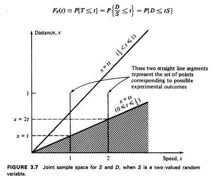
Examining Figure 3.7, we see that the straight line x = ts
intersects both "lines" of the sample space for 0 < t < 1/2. So,
for those values of t, we have

The "1/2"'s arise from integrating left to right across the
impulses; the FD(·) terms arise from integrating from x = 0 to x
= ts at
s = 1 and s = 2. Since from Example 1, (3.1), we know that

Once t exceeds 1/2 in value, the sweep of the line x = ts no longer
picks up additional probability from the "line impulse" at s =
2. So, for 1/2 < t  1, FT(t) =1/2[1 - (1 - t)2] + 1/2. Thus, combining
results, the answer to our problem is
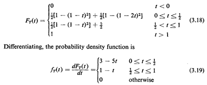
This pdf is sketched in Figure 3.8. Note the discontinuity in
slope at t=1/2.
This is not unusual in practice; in fact, one often comes across
problems in which the derived pdf is discontinuous (in
value) at one or more points. Points of discontinuity, either in
value or slope, usually correspond to "switchover points"
in the original sample space in which the summation or integral
for accumulating probability for the cdf switches over to
some new functional form. Switchovers often occur when the region
of accumulated probability changes in geometric form,
such as occurred at t=1/2 in the example.
While we have completed our derived distribution work on this
problem, there is one additional issue that we wish to
address and that deals with expected values of random variables.
Here the expected value of T is
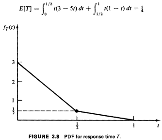
We may wish to calculate the expected value simply by working in
the (D, S) sample space. Because of independence, if T =
h1(D)h2(S), then
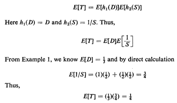
as calculated previously, This is an illustration of the
following general principle:
If one only desires expected values and not the complete
probability law of a function of random variables, it is usually
computationally easier to work directly in the original sample
space to compute the expected values.
There is a second general principle we can illustrate with this
example. When asked to calculate E[T], one may be
tempted to say that

Clearly, this is not correct, the answer being about 11 percent
less than the correct answer. The error lies in assuming that
E[1/S] = 1/E[S].
In general, the expected value of a function of a random variable
is not equal to the function evaluated at the expected value
of the random variable.
In this case one can prove mathematically that for any
nonnegative random variable S,

Hence, using (E[D]/E[S]) to estimate E[T] in such a case results
in an optimistically low estimate of average travel time. In
a practical sense these relations imply that an urban service
agency cannot infer that, say, a 20-mile/hr average response
speed and a 1-mile average travel distance imply a 3-minute
average travel time. On the contrary, the average inverse speed
could be, say, 0.10 hour/mile; in such a case if travel distance
and travel speed are independent, the average travel time is 6
minutes, not 3 minutes.
Further work: Problem 3.5.
Example 3: Rayleigh Distribution
To this point our derived distribution examples have dealt with
sample spaces in which all random variables had finite
maximum and minimum values. This is not a necessary requirement,
and many derived distribution problems, such as the
case considered here, allow one or more random variables to
assume infinitely large (positive or negative) values.
Suppose an urban vehicle is located at (X0, Y0). An automatic
vehicle location (AVL) system utilizes one of the several
available technologiesz to estimate the location of the vehicle.
Such an application is relevant in police departments,
taxicab services, maintenance services, and numerous other urban
services. Suppose that the estimated position of the
vehicle is given by
X = X0 + Xe
Y = Y0 + Ye
where (X0, Y0) represent the true position coordinates of the
vehicle and (Xe, Ye) are the additive error terms due to imperfect
resolution. For certain AVL technologies it makes sense to assume
that Xe and Ye are independent, zero-mean Gaussian
random variables:

where the standard deviation  specifies the resolution of the
system. It now makes sense to examine properties of the
"radius of error" specifies the resolution of the
system. It now makes sense to examine properties of the
"radius of error"

Solution
To derive the probability law of R we work in the (Xe, Ye) sample
space, which is the entire plane (Figure 3.9), and utilize
the joint (Xe, Ye) pdf, which is (by independence)

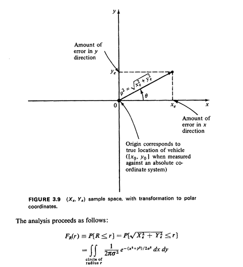
Because of the circular symmetry of the situation, we find it
easier to evaluate this integral by changing to polar
coordinates  and and  , where , where

These relationships are shown in Figure 3.9. Since the
infinitesimal area to be integrated changes from dx dy to  d
d d d ,
we can write ,
we can write

Carrying out the final integration, we find that
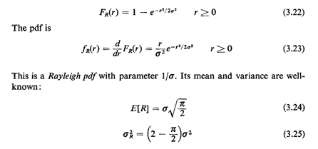
Notice that this pdf behaves as we might expect intuitively: it
starts at zero at r = 0 and grows monotonically to a maximum
(which occurs at r = ) and then decreases monotonically in an
exponential way according to r2 ) and then decreases monotonically in an
exponential way according to r2
Among other applications, the Rayleigh probability law arises in
physics in various scattering experiments and in
communication theory in the modeling of noise over a
communication channel. We have now seen how it arises as a
derived distribution in an urban vehicle location context.
There is an alternative way of deriving the Rayleigh pdf directly
without first finding the cdf. The method is useful in
other applications, as well, in which it is easy to make
infinitesimal probability arguments. However, when in doubt, we
always prefer to resort to the never-fail cdf method. The direct
method proceeds as follows : since a pdf has a probability
meaning only if it is integrated, we "integrate" fR(r) over the
infinitesimal interval [r, r + dr),

Again because of circular symmetry, we change to polar
coordinates  and 6, with and 6, with
 = r and d = r and d = dr, thereby obtaining = dr, thereby obtaining
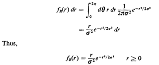
as previously derived. We used such an infinitesimal argument
when showing in Section 2.12 that the Ith-order interarrival
time of a Poisson process has an Ith-order Erlang pdf. However,
again we caution those computing derived distributions
that this "infinitesimal" method for finding the pdf directly is
fraught with potential pitfalls and difficulties for all but the
simplest problems. Thus, the never-fail cdf method remains our
primary tool for deriving distributions.
Further work on A VL position estimation errors: Problems 3.6 and
3.7.
Example 4: Ratio of Right Angle to Euclidean Distance Metrics
As another example of deriving distributions of random variables,
we consider a problem that arises in transportation
systems (e.g., "dial-a-ride" systems, taxicab systems), emergency
services (fire, police, and ambulance), and other
municipal systems having mobile units. The problem deals with the
"penalty" in travel distance incurred by a mobile unit
while traveling a grid of streets, compared to a helicopter or
other unit that could travel "as the crow flies."
If the mobile unit is located at (x1, y1) and is traveling along
a shortestdistance path to (x2, y2) perhaps to pick up a
passenger, then the right-angle distance between the points is
d = |x1 - x2| + |y1 - y2|
If street directions are parallel to the coordinate axes, the
right-angle distance (also called Manhattan, metropolitan, or
rectangular distance) is a good approximation for the actual
travel distance covered. 3
Of interest in designing computer dispatching algorithms and in
developing planning models, the ratio of the right
angle to the Euclidean distance provides insight as to the extra
distance traveled because of the requirement of driving on
streets. For instance, if one knew the average value of this
ratio, then in a computer dispatching algorithm it might be
acceptable to estimate the travel distance as the product of this
average value and the Euclidean distance, the latter being
obtained easily from a file of (x, y) coordinates.
Consider two points (X1, Y1) and (X2, Y2),
corresponding to the
trip origin and destination, respectively, defined
relative to any fixed coordinate system. Let  (0
(0  
  /2) be
the angle at which the directions of travel are rotated with
respect to the straight line connecting the two points (see
Figure 3.10). Given /2) be
the angle at which the directions of travel are rotated with
respect to the straight line connecting the two points (see
Figure 3.10). Given  , the right-angle travel distance between
(X1, Y1) and X1, Y1) is , the right-angle travel distance between
(X1, Y1) and X1, Y1) is

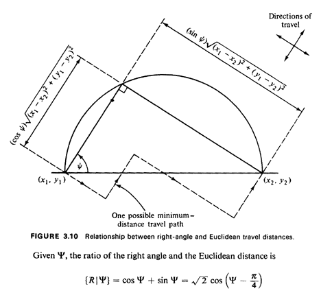
We wish to derive the cdf of R using the never-fail method,
making reasonable assumptions about the probabilistic
behavior of  . .
Solution
Here we are deriving the distribution of one continuous random
variable which is expressed as a function of another
continuous random variable (i.e., a "one-to-one" transformation).
The cdf of R is

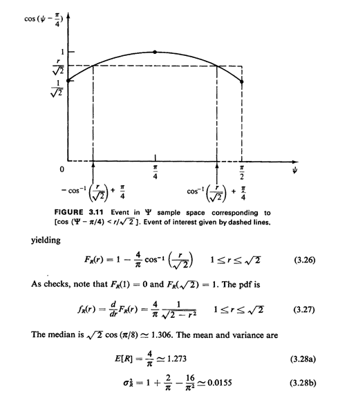
The event corresponding to (R  r) in the r) in the
 sample space is shown
in Figure 3.11. Now in a large, uniform city it makes
sense to assume that sample space is shown
in Figure 3.11. Now in a large, uniform city it makes
sense to assume that  is uniformly distributed over [0, is uniformly distributed over [0,  /2].
(Why?) We call this an isotropy assumption, meaning
sameness regardless of direction. Given the isotropy assumption,
we can integrate the pdf of /2].
(Why?) We call this an isotropy assumption, meaning
sameness regardless of direction. Given the isotropy assumption,
we can integrate the pdf of  over the event indicated in
Figure 3.11 to obtain over the event indicated in
Figure 3.11 to obtain

Thus, "on the average" the mobile unit travels about 1.273 times
the Euclidean
distance (given the model assumptions). Since  = 0.0155, the ratio
 R/E[R], the coefficient of variation, is only 0.098, meaning
that the estimate of 4/
 for E[R] is quite robust.
A reasonable "test" of the right-angle distance metric would be
to compare the empirical distribution of ratios of
recorded travel distances and corresponding Euclidean distances
to FR(·) and to compare the empirically found average R to
1.273. for E[R] is quite robust.
A reasonable "test" of the right-angle distance metric would be
to compare the empirical distribution of ratios of
recorded travel distances and corresponding Euclidean distances
to FR(·) and to compare the empirically found average R to
1.273.
Further work: Problem 3.8 {deriving E[R] and  without
FR(·)};
Problems 3.9 and 3.10 (alternatives to the isotropy assumption). without
FR(·)};
Problems 3.9 and 3.10 (alternatives to the isotropy assumption).
Example 5: Quantization Model
As a final detailed example of a derived distribution problem, we
consider a situation in which two continuous random
variables give rise to one discrete random variable. This 2-to-l
transformation arises due to quantization of odometer
readings in urban vehicles. The same analysis applies in other
quantization settings, for instance in cases where successive
event times are quantized.
Assume that we are running an experiment to estimate the
distribution of distance traveled by taxicabs, where distance
D  miles traveled from the moment of
dispatch to arrival at the
address of the caller miles traveled from the moment of
dispatch to arrival at the
address of the caller
All we have available experimentally are recorded travel
distances, which are quantized as 0 miles, I mile, 2 miles, and so
on. We wish to examine the quantitative effects of such
truncation. Quite clearly, the same model could be used for
studying
response distances of emergency vehicles, "paid" trips of
taxicabs, trips of dial-a-ride vehicles, etc.
For a journey of length D, the recorded travel distance equals
the sum of D and the accumulated odometer mileage at the
moment of dispatch since the last odometer reading change, the
sum truncated to the largest integer not exceeding the sum.
For instance, if the vehicle had traveled 0.9 mile since the last
reading change and then traveled 1.2 miles to the address of
the caller (following dispatch), the recorded mileage would be
the largest integer not exceeding (0.9 + 1.2) = 2.1, which is
2 (miles). If, however, the noninteger accumulated odometer
mileage at the moment of dispatch had been 0.6 rather than
0.9, the recorded mileage would be the largest integer not
exceeding (0.6 + 1.2) = 1.8, which is I mile. In the first case,
the
odometer's mileage reading had changed twice; in the second,
once. As examples will clearly demonstrate, the recorded
travel distance can either underestimate or overestimate the
actual travel distance by as much as I mile.
Solution
Random Variables
There are two key random variables that give rise to the
quantized distance random variable:
D  actual travel distance actual travel distance
  accumulated noninteger
odometer mileage at the moment
of dispatch (a random variable distributed over [0, 1)) accumulated noninteger
odometer mileage at the moment
of dispatch (a random variable distributed over [0, 1))
If we let the quantized distance random variable be
K  recorded mileage for the journey recorded mileage for the journey
Then K is a function of D and  : :

Here we have a discrete random variable expressed as a function
of two continuous random variables. If we have the joint
probability law for D and  ),
we would like the probability law
for K. ),
we would like the probability law
for K.
Joint Sample Space
The (D,  ) sample space is the infinite strip of
width 1 (0 < D < ) sample space is the infinite strip of
width 1 (0 < D <
 , 0 , 0 

 1), shown in Figure 3.12. Without yet
assigning a probability law over this sample space, we have
performed in Figure 3.12 the "work" required to find the sets of
points in the sample space that give rise to different values 1), shown in Figure 3.12. Without yet
assigning a probability law over this sample space, we have
performed in Figure 3.12 the "work" required to find the sets of
points in the sample space that give rise to different values
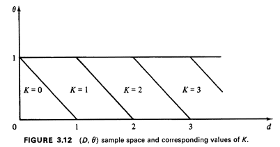
of the random variable K. We illustrate the derivation of one of
the "45° lines" partitioning the sample space. Suppose that
the experimental value for D lies between 1 and 2 (i.e., 1  d
d 2). Then, for "sufficiently small" 2). Then, for "sufficiently small"  , K will equal 1;
otherwise, K will equal 2. The switch from K = 1 to K = 2 will
occur at the point at which d +
  = 2. Thus, the switch occurs
along the line = 2. Thus, the switch occurs
along the line

Joint Probability Distribution
Without knowing the exact distribution for D, we can make some
further progress in our analysis of the effects of
quantization. From physical considerations, the following
assumptions seem reasonable:
- The random variables D and
 are independent. are independent.
-
 is uniformly distributed over [0,1]. (Why?) is uniformly distributed over [0,1]. (Why?)
Thus, we will limit our knowledge of the joint (D, )pdf to say
that it takes the following form: )pdf to say
that it takes the following form:

Working in the Joint Sample Space
Since entire subregions of the (D,  )
sample space give rise to
exactly one value of K, we can deal directly with the pmf
for K, not the cdf. Given the assumptions regarding fD, )
sample space give rise to
exactly one value of K, we can deal directly with the pmf
for K, not the cdf. Given the assumptions regarding fD,  (d,
(d, )
above, if the cdf for D is known, say FD(·), the probability
mass function for K is readily computed: )
above, if the cdf for D is known, say FD(·), the probability
mass function for K is readily computed:

Thus, any statistical procedure using experimental data to
estimate E[K] should also yield an (unbiased) estimate of E[D].
For such a procedure to remain unbiased, it is necessary that
zero-mileage journeys be recorded and used in the statistical
tabulations.
Question: Given the foregoing analysis, can one lump together
recorded mileages quantized in tenths of miles with those
quantized in miles?
Furtherwork: Problem 3.11 [for a proof of (3.31)]; Problem 3.12
(for an application of these ideas to time measurements).
1 Typical empirical relationships found among speed, distance, and
time are described later in this chapter.
2 See, for example, R. C. Larson, K. W. Colton, and G. C. Larson,
"Evaluating an Implemented AVM System: The St. Louis
Experience (Phase I)," Public Systems Evaluation, Inc.,
Cambridge, Mass., 1976.
3 See Problems 3.24 and 3.25 for realistic variations to the
right-angle distance (due to discreteness of streets and one-way
streets).
|


 X1
X1  I
I X2
X2 X1
X1 1, 0
1, 0  X2
X2  1).
1).


 X2; case 2: X1 < X2
. For the first case,
D = X1 - X2 and experimental values x1 and x2
of X1 and X2,
respectively, must lie between the line x2 = x1 and x2
= xI - y
(Figure
3.1). For the second case, D = X2 - X1, and experimental values
of X1 and X2 must lie between the line x2 = x1
and x2 = xI + y.
Consideration of these two cases gives rise to the shaded region
in the sample space in Figure 3.1. Once we have
determined such a region, we have identified the set of points
corresponding to the event of interest: [D < y), thereby
completing step a of the never-fail method. This is often the
most difficult part of a derived distribution problem. Note that
determination of this region in no way depended on the joint pdf
for X1 and X2; thus, the "work" invested to this point could
be applied to several alternative models, each with its own joint
pdf for X1 and X2.


 ?]
?]


 y) is the line segment of length 2y
centered at X1=1/2. Integrating the (uniform) pdf of X1, we have
FD'(y) =P{D'
  y)=
P{ | X - 1/2 |
  y)= 2y (O
  y
y
 1/2). Thus, the pdf of D'is


 r, we again consider two
cases: case 1: X1
  X2; case 2: X1
 X2. For case 1, Max (X1,
X2) = X1 and the event Max (X1, X2)
 r corresponds to
the set of points to the left of the line x1 = r (Figure 3.4).
Similarly, for case 2, Max (X1, X2) = X2 and the event Max (X1,
X2)
  r corresponds to the set of points below the line X2 =
r. Combining these two cases, the event Max (X1, X2)
  r
corresponds to the square of area r2 shown in Figure 3.4.
 1, we again
consider case 1: X1
  X2, and case 2: X1
  X2. For
case 1, Min (X1, X2) = X2 and the event Min
(X1, X2)
  1
corresponds to the set of points below the line x2 = 1 (Figure
3.4). For case 2, Min (X1, X2) = X1 and the event Min (X1, X2)
 1 corresponds to the set of points to the left of the line x1
= 1. Combining these two cases, the event Min (X1, X2)
  1
corresponds to the L-shaped region shown in Figure 3.4.

 r, L
r, L
 l}, shown in the crosshatched
region in Figure 3.4. We have now completed step a of the
never-fail method,


 tS) in the (D, S) sample space is
shown in Figure 3.6. In principle, all we need do is
integrate the joint D, S pdf over this region for each value of t
to obtain the cdf for T, FT(t). 1


 1, FT(t) =1/2[1 - (1 - t)2] + 1/2. Thus, combining
results, the answer to our problem is


 specifies the resolution of the
system. It now makes sense to examine properties of the
"radius of error"


 and
and  , where

 d
d d
d ,
we can write


 ) and then decreases monotonically in an
exponential way according to r2

 and 6, with
 = r and d
 = dr, thereby obtaining

 (0
(0 


 /2) be
the angle at which the directions of travel are rotated with
respect to the straight line connecting the two points (see
Figure 3.10). Given
  , the right-angle travel distance between
(X1, Y1) and X1, Y1) is


 .
.
 r) in the
 sample space is shown
in Figure 3.11. Now in a large, uniform city it makes
sense to assume that
  is uniformly distributed over [0,
  /2].
(Why?) We call this an isotropy assumption, meaning
sameness regardless of direction. Given the isotropy assumption,
we can integrate the pdf of
  over the event indicated in
Figure 3.11 to obtain


 = 0.0155, the ratio
 R/E[R], the coefficient of variation, is only 0.098, meaning
that the estimate of 4/
 for E[R] is quite robust.
A reasonable "test" of the right-angle distance metric would be
to compare the empirical distribution of ratios of
recorded travel distances and corresponding Euclidean distances
to FR(·) and to compare the empirically found average R to
1.273.
 without
FR(·)};
Problems 3.9 and 3.10 (alternatives to the isotropy assumption).
 miles traveled from the moment of
dispatch to arrival at the
address of the caller
 actual travel distance
 accumulated noninteger
odometer mileage at the moment
of dispatch (a random variable distributed over [0, 1))
 recorded mileage for the journey
 :
:

 ),
we would like the probability law
for K.
 ) sample space is the infinite strip of
width 1 (0 < D <
 , 0
, 0 

 1), shown in Figure 3.12. Without yet
assigning a probability law over this sample space, we have
performed in Figure 3.12 the "work" required to find the sets of
points in the sample space that give rise to different values

 d
d 2). Then, for "sufficiently small"
  , K will equal 1;
otherwise, K will equal 2. The switch from K = 1 to K = 2 will
occur at the point at which d +
  = 2. Thus, the switch occurs
along the line

 are independent.
 is uniformly distributed over [0,1]. (Why?)
 )pdf to say
that it takes the following form:

 )
sample space give rise to
exactly one value of K, we can deal directly with the pmf
for K, not the cdf. Given the assumptions regarding fD,
  (d,
(d, )
above, if the cdf for D is known, say FD(·), the probability
mass function for K is readily computed:


