3.3.1 Buffon's Needle Experiment
A famous "needle-throwing" experiment first proposed by Buffon in
1777 provides a good example of
probabilistic modeling from a geometrical point of view [BUFF
771. Suppose we have a large flat surface that has
been ruled with a series of equidistant parallel lines separated
by a distance d. (For instance, one might imagine this
to be the alternating red and white striped field of the American
flag.) An experimenter throws a needle of length l
 d
d "at random" onto the surface and we wish to compute the
probability that the needle intersects one of the parallel
lines (e.g., lies on both red and white stripes of the flag). We
suppose that the surface is large enough so that the
needle always lands on it and that boundary effects are
negligible. d
d "at random" onto the surface and we wish to compute the
probability that the needle intersects one of the parallel
lines (e.g., lies on both red and white stripes of the flag). We
suppose that the surface is large enough so that the
needle always lands on it and that boundary effects are
negligible.
To model this experiment, just as with other probabilistic
experiments, there are four things we must do:
STEP 1: Define the random variables of interest.
STEP 2: Identify the joint sample space.
STEP 3: Determine the joint probability distribution over the
sample space.
STEP 4: Work within the sample space to determine the answers to
any questions about the experiment.
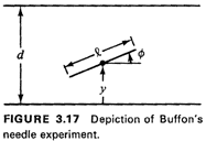
- Random variables. Any experimental outcome is fully described
by the position of the needle on the
surface. A convenient depiction of this position is given by two
random variables (see Figure 3.17):
Y = distance from the center of the needle to the
closest of the equidistant parallel lines
 = angle of the needle, measured
with respect to the parallel lines = angle of the needle, measured
with respect to the parallel lines

With the position random variables defined in this way, we
clearly have 0  Y Y
 d/2 and
0 d/2 and
0  
  .
This choice of random variables is motivated in part by symmetries that can be
exploited and in part by the simple probability laws
that govern their behavior. Other sets of random variables could
be selected, some that would lead to tractable
analyses and some that would not. For instance, we could define Y
to be the distance from the center of the needle to
the next "southern" parallel line (assuming that the lines run
east-west). In this case 0 .
This choice of random variables is motivated in part by symmetries that can be
exploited and in part by the simple probability laws
that govern their behavior. Other sets of random variables could
be selected, some that would lead to tractable
analyses and some that would not. For instance, we could define Y
to be the distance from the center of the needle to
the next "southern" parallel line (assuming that the lines run
east-west). In this case 0  Y Y
 d, and the analysis
follows very closely the analysis given below. However, we could
also define the position of the needle by the (x,y) coordinates of its two end points; this
would lead to an unnecessarily complicated analysis. In analyzing an
experiment, the efficient selection of a reasonable set of random
variables often comes only with modeling
experience. d, and the analysis
follows very closely the analysis given below. However, we could
also define the position of the needle by the (x,y) coordinates of its two end points; this
would lead to an unnecessarily complicated analysis. In analyzing an
experiment, the efficient selection of a reasonable set of random
variables often comes only with modeling
experience.
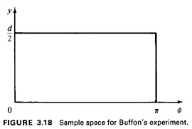
- Joint sample space. For the position random variables we have
selected, the joint (Y,
 ) sample space
corresponds to the rectangle 0 ) sample space
corresponds to the rectangle 0  y y
 d/2,
0 d/2,
0  
 (Figure 3.18).

- Joint probability distribution. To determine the joint
probability density function fY,
 (y, (y,
 ) we must
interpret the words "at random,"
describing the throwing mechanism. This is
often not an easy thing to do, as the example in the next section will
illustrate. In the absence of other information, it is plausible
to assume here that the angular position of the needle
is uniformly distributed between 0 and ) we must
interpret the words "at random,"
describing the throwing mechanism. This is
often not an easy thing to do, as the example in the next section will
illustrate. In the absence of other information, it is plausible
to assume here that the angular position of the needle
is uniformly distributed between 0 and  , and thus the marginal
pdf for the angle is

Similarly, it is reasonable to assume that the location of the
center of the needle is uniformly distributed, implying that

To obtain the joint pdf, fy, (· , ·)it would be "nice" if
 and Y
were independent, for then the joint pdf would
simply be the product of the two marginals. Indeed, in this case,
there is no reason to assume that knowing the
needle's angle would affect one's knowledge about its center
position or conversely, and thus the independence
assumption can be invoked. Thus, and Y
were independent, for then the joint pdf would
simply be the product of the two marginals. Indeed, in this case,
there is no reason to assume that knowing the
needle's angle would affect one's knowledge about its center
position or conversely, and thus the independence
assumption can be invoked. Thus,

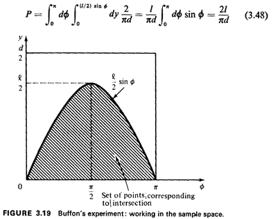
4. Working in the joint sample space. We are asked for the
probability that the needle intersects one of the
parallel lines. To answer this question, all we need do is
identify the set of points in the joint (Y,  ) sample
space that corresponds to "intersection of a parallel line" and
integrate the joint pdf over that set of points to
obtain the desired probability. To do this, we must define
"intersection of a parallel line" in terms of the random
variables in the sample space.
By examining Figure 3.17, it is clear that intersection will
occur if "y is sufficiently small for a given angle ) sample
space that corresponds to "intersection of a parallel line" and
integrate the joint pdf over that set of points to
obtain the desired probability. To do this, we must define
"intersection of a parallel line" in terms of the random
variables in the sample space.
By examining Figure 3.17, it is clear that intersection will
occur if "y is sufficiently small for a given angle  ."
Assuming the situation shown in Figure 3.17, the coordinate of
the lower end of the needle is y - (1/2) sin ."
Assuming the situation shown in Figure 3.17, the coordinate of
the lower end of the needle is y - (1/2) sin  . If
this coordinate is negative, intersection will occur. Thus,
intersection occurs for all points in the (Y, . If
this coordinate is negative, intersection will occur. Thus,
intersection occurs for all points in the (Y,  ) sample
space satisfying the inequality y ) sample
space satisfying the inequality y  (l/2) sin (l/2) sin
 . Integrating
over this set (see Figure 3.19), we obtain the desired
probability: . Integrating
over this set (see Figure 3.19), we obtain the desired
probability:

A somewhat remarkable property of this result is that it contains
a fundamental constant of nature,  . If one
threw needles many times (and independently) at a lined surface,
one could estimate . If one
threw needles many times (and independently) at a lined surface,
one could estimate  .
Exercise 3.4-. Buffon's Needle, Another Way Redo this analysis
assuming that the random variable Y is the
distance from the center of the needle to the next "southern"
parallel line (so that 0 .
Exercise 3.4-. Buffon's Needle, Another Way Redo this analysis
assuming that the random variable Y is the
distance from the center of the needle to the next "southern"
parallel line (so that 0  Y Y
 d).
Exercise 3.5: Buffon's Longer Needle Solve the Buffon needle
problem for the case in which the needle is
unrestricted in length, (This requires an analysis of the case I
> d.) d).
Exercise 3.5: Buffon's Longer Needle Solve the Buffon needle
problem for the case in which the needle is
unrestricted in length, (This requires an analysis of the case I
> d.)
|


