


3.5.1 Response Distance of an Ambulette, RevisitedAs in Example I of Section 3. 1, suppose that X1 and X2 are independent and uniformly distributed over the interval [0, a]. We want the mean travel distance, which we call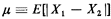
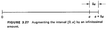
Clearly, this expected value can be obtained easily by our earlier (direct) methods, but this simple example will illustrate the basic idea of Crofton's method. We add to the interval [0, a] an increment of length
following four mutually exclusive events: 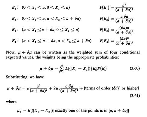
The key to Crofton's method is that it isolates one of the points in the infinitesimal interval, thereby yielding a quantity  1, which is the mean value of the random variable, given
that one of the points is located in the
infinitesimal interval. This quantity is usually easier to
compute than (since one of the points is "pinned down"). 1, which is the mean value of the random variable, given
that one of the points is located in the
infinitesimal interval. This quantity is usually easier to
compute than (since one of the points is "pinned down").
In this problem it is obvious that
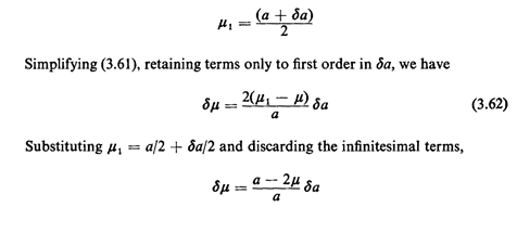
which yields the differential equation 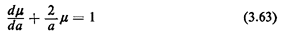
As with most differential equations, this one has a homogeneous and a particular solution. The homogeneous solution is = Kh/a2
for some constant K, Here K,
must be set equal to zero, since
otherwise becomes infinitely large as a approaches zero, a
result obviously not physically
possible (since  a). Motivated by physical considerations
(and the result of scaling random
variables-Section 3.1), we propose as a particular solution =
Kpa. Substituting in (3.63), we find K,
thus corroborating our earlier result of Example 1. a). Motivated by physical considerations
(and the result of scaling random
variables-Section 3.1), we propose as a particular solution =
Kpa. Substituting in (3.63), we find K,
thus corroborating our earlier result of Example 1.
Examining the derivation, we could retain
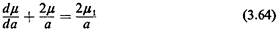
Note that this differential equation has been derived considering only the geometry of the region R and the uniform probability laws of X1 and X2; in particular, the specific form of the function whose expected value is 1 has not been considered in the
derivation.
For example, if we identify 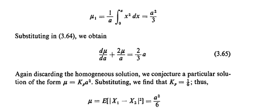
Combining our two results, we find for the variance 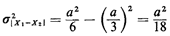
In general, Crofton's method can be used to find any of the moments of the random variable of interest. In many cases we can extend these ideas to find the probability
distribution of the random variable. We do this
by invoking a set indicator random variable. A random variable XA
is said to be an indicator random variable for the
set A if
The utility of the set-indicator random variable derives from its simplicity (only two possible values) and the fact that In our continuing example, suppose that we define the
set-indicator random variable as follows:
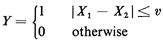
Now the expected value of Y will equal the probability that |X1 - X2|  D
is less than or equal to v; thus, in this case, D
is less than or equal to v; thus, in this case,
This is the essential relationship one requires to apply Crofton's ideas to deriving probability laws of functions of random variables (very special random variables, to be sure). Hence, solving Crofton's problem in this instance provides us with the cdf for the random variable |X1 - X1| = D. Here 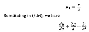
But this is equivalent to 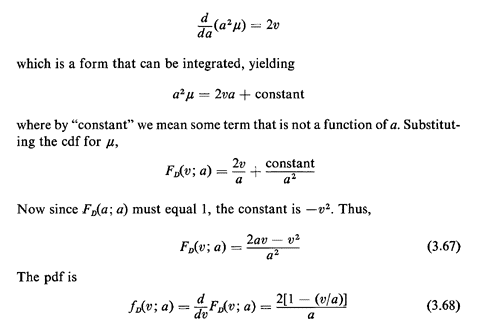
which confirms earlier results (Example 1). Crofton's method can be generalized to situations in which there
are N points distributed independently and
uniformly over R. 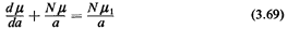
6Technically, given the definition of 1
in (3.61), 1 on the
right hand side of (3.64)
should be replaced with  .
For simplicity of notation, we
have chosen to ignore
the infinitesimal term involved since it plays no role in the
resulting differential equation. .
For simplicity of notation, we
have chosen to ignore
the infinitesimal term involved since it plays no role in the
resulting differential equation.
|
 a, as shown
in Figure 3.27. We now consider the problem
in which X1 and X2 are independent and distributed in the same
way as before, but over the larger interval [0, a +
a, as shown
in Figure 3.27. We now consider the problem
in which X1 and X2 are independent and distributed in the same
way as before, but over the larger interval [0, a +