4.8.2 Queueing Systems with No Waiting Space
One of the few examples of
"difficult" queueing systems
for which exact results exist are M/G/m systems with no waiting
space. Instances in which
these models are, at least approximately, applicable in urban
operations research are
common and usually involve emergency services.
For example, a few years
ago the following
situation came under review in one of our major cities. A small
fleet of
hospital-affiliated ambulances were being used as the primary means
of transporting
emergency patients to local hospitals. At those times when all
ambulances were busy,
a back-up fleet of "ambulettes" run by the police department
of that city was
pressed into service. No queue was allowed to form for service by
the hospital-affiliated
ambulances. It was generally believed by EMS planners that police
ambulettes provided
inferior service (a belief that was apparently shared by many city
residents). As a
result, it was decided to increase the size of the
hospitalaffiliated fleet and it was
desired to determine the minimum number of active
hospital-affiliated ambulances that
would be necessary to assure that:
P{a random emergency patient must be served by a police
ambulette} f f
where f is a threshold probability (0 < f
< 1).
Calls for emergency
ambulance service arise in
a Poisson fashion in time and the service times for calls (involving
a trip to the
location of the call, some time spent there, and, finally,
transportation to a
hospital) are random variables with "general" pdf's.
Therefore, in the presence
of a fleet of m hospital-affiliated ambulances, the fraction of
calls serviced by police
ambulettes is equal to the probability, Pm
, that all m hospital
ambulances are busy as
given by a M/G/m queueing model with no waiting space.
It has been shown (see,
for instance, [GROS
74]) that, quite remarkably, the expressions for the steady-state
probabilities for this
M/G/m case are identical to those for the corresponding
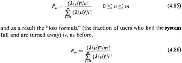
M/M/m system. Thus, as in
(4.57), we have

To get back to our
example, the number of
hospital ambulances needed is the smallest m such that
Pm  f. It is
particularly surprising that (4.85) and (4.86) depend only on the
mean of the service
times.
M/G/ queueing
system. The M/G/ queueing
system. The M/G/ queueing system can now be viewed as a
special case of the
M/G/m system with no waiting space, by taking the limiting value m queueing system can now be viewed as a
special case of the
M/G/m system with no waiting space, by taking the limiting value m
  for
the latter system.
Thus, we can use directly our last result. Replacing m by for
the latter system.
Thus, we can use directly our last result. Replacing m by  in (4.85), we have in (4.85), we have

As one would expect
[since (4.85) is identical
to (4.57)], this expression is the same as (4.50) for the M/M/ system. As with the
M/M/ system. As with the
M/M/ system, we also have
  = =  / / , ,  = 1/ = 1/ , and , and  q
= q
=  q,
= 0 in this case. q,
= 0 in this case.
It is instructive to
derive (4.87) directly
because in the process one can also derive the time-dependent
probabilities Pn(t)
of having n users in the M/G/ system at time t assuming that the system
was empty at t = 0.
In the following we shall use Fs(s) to
denote the cdf for
the service times and also use the fact that system at time t assuming that the system
was empty at t = 0.
In the following we shall use Fs(s) to
denote the cdf for
the service times and also use the fact that

Exercise4A Show that the above relationship holds for any
random variable S that
assumes only non-negative values. [Hint: It is easier to work
initially with a discrete
random variable.]
We define
1. Pn(t)  P{at time t there are exactly n users
being serviced}. P{at time t there are exactly n users
being serviced}.
2. Pn  lim t lim t  Pn(t).
We wish to prove the following:
[Note from (4.88) that, for any given t, P.(t) is a Poisson pmf.]
Proof: Let the queueing system be empty at t = 0 and let
Pn(t | k) ~ P{at time t there are
exactly n users being
served | exactly k arrivals in [0, t]}
Then, since arrivals occur according to a Poisson process,

But, as we have seen in Chapter 2, if there are exactly
k arrivals from a
Poisson process in [0, t], the unordered arrival times are
uniformly, independently
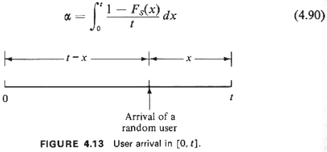
distributed over [0, t]. So, we now consider a random user arriving
in the interval [0, t]
(see Figure 4.13). If the random user arrives with x more time left
in [0, t], the
probability that he is still being serviced at t is [1 - F,(x)]. But
the unconditional
probability he arrives in [t - x, t - x + dx] is dx/t. Thus, the
probability that a random
user who arrives any time in [0, tl is still being serviced at time
t is

We now use the fact that the unordered arrival times are
independent. Given k arrivals
in [0, t], the probability that there are n customers being serviced
at t (n  k) is
k) is

Substituting (4.90) and (4.91) into (4.89), we obtain
(4.88)-after some algebraic
manipulation. The steady-state result (4.87) is derived just by
letting t   in
(4.88). in
(4.88).
As we have already noted
earlier, in order to
apply a M/G/ (or M/M/ (or M/M/ )
model, it is not really
necessary to have an infinite number of servers. In practice, all
that is needed is that
the actual number of servers be sufficiently large or that workload
be sufficiently small
so that queues almost never form. Fire department operations, for
example, possess this
characteristic. It is highly unlikely that in a major city there
will ever be insufficient
fire engines or fire ladders to dispatch to a major fire; for if the
fire stations in a
given area run out of fire companies as a result of one or more
multiple alarm fires, then
other fire companies are dispatched to the scene, first from
neighboring stations and
eventually, if necessary, from nearby cities or communities.
Assuming then that fire
alarms in a region are generated according to a Poisson process,
service times for
different fire alarms are statistically independent and identically
distributed, fire
alarm rates and service rates are constant in time, and an infinite
number of
fire-fighting units are available, one can use the M/G/ )
model, it is not really
necessary to have an infinite number of servers. In practice, all
that is needed is that
the actual number of servers be sufficiently large or that workload
be sufficiently small
so that queues almost never form. Fire department operations, for
example, possess this
characteristic. It is highly unlikely that in a major city there
will ever be insufficient
fire engines or fire ladders to dispatch to a major fire; for if the
fire stations in a
given area run out of fire companies as a result of one or more
multiple alarm fires, then
other fire companies are dispatched to the scene, first from
neighboring stations and
eventually, if necessary, from nearby cities or communities.
Assuming then that fire
alarms in a region are generated according to a Poisson process,
service times for
different fire alarms are statistically independent and identically
distributed, fire
alarm rates and service rates are constant in time, and an infinite
number of
fire-fighting units are available, one can use the M/G/ model to estimate the
distribution of the number of
fire-fighting units which are busy at any one time in an
area. Although the
validity of some of the assumptions above may be questioned, the
results provided by such
a model 9 [CHAI 71] have been shown to
provide excellent
approximations to the true distribution [IGNA 78]. model to estimate the
distribution of the number of
fire-fighting units which are busy at any one time in an
area. Although the
validity of some of the assumptions above may be questioned, the
results provided by such
a model 9 [CHAI 71] have been shown to
provide excellent
approximations to the true distribution [IGNA 78].
9 The referenced model, due to J. Chaiken, is a modified
M/G/ model which
accounts for the fact that
two or more fire units are often simultaneously dispatched to a
fire alarm. model which
accounts for the fact that
two or more fire units are often simultaneously dispatched to a
fire alarm.
|