5.7 SPATIAL DISTRIBUTION OF BUSY SERVERSIn some situations we would like to know the spatial distribution of servers busy at the scene of service requests. For instance, we may wish to analyze a dispatching policy which may interrupt a server busy on low-priority service in order to send him or her to a nearby higher-priority request; in such a case we would need to know the distribution of travel time to the nearest busy server. Or, in police applications, since police presence is said to deter crime, we may wish to know the spatial distribution of busy servers (as well as available servers) because a parked patrol car also acts as a visible deterrent; we may wish to alter this distribution, if possible, by adjusting our spatial prepositioning policies (e.g., beat designs). We examine this question using the theory of M / G / Consider, then, a spatially distributed service system in which:
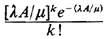
Then, according to (4.87), in the steady state the probability that
there are k busy service units in any subregion of area A
This result says that, regardless of the method of prepositioning the
units, the busy servers are distributed as a spatial Poisson
process with parameter ( |
 queues (cf. Section 4.8). The assumption of an
infinite number of servers implies that the actual number of servers is
sufficiently large or that workload is sufficiently small so that queues
almost never form.
queues (cf. Section 4.8). The assumption of an
infinite number of servers implies that the actual number of servers is
sufficiently large or that workload is sufficiently small so that queues
almost never form. Ao requests per hour.
 -1 = average time to service a
request (general service time pdf).
-1 = average time to service a
request (general service time pdf).
 Ao is
Ao is