


6.2.2 Shortest Paths between All Pairs of Nodes [4(i, j) > O]It is very often the case that the shortest paths between all pairs of nodes in a network are required. An obvious example is the preparation of tables indicating distances between all pairs of major cities and towns in road maps of states or regions, which often accompany such maps. Another example is the calculation of the distances between all pairs of "atoms" in connection with the use of the hypercube model of Section 5.4. This type of computation, as we shall see later in this chapter, is also virtually invariably required in all urban service system problems related to the location of urban facilities or to the distribution or delivery of goods. It is therefore important to have available a highly efficient method for obtaining these shortest paths. One obvious approach is the repeated application of Algorithm 6.1 of the previous section, setting each node of the graph, in succession, as the source node and thus finding the shortest-path tree associated with each and every one of the graph's nodes. Another elegant and simpleto-program approach is generally attributed to Floyd [FLOY 62]. Floyd's algorithm is simple to describe, but its logic is not particularly easy to grasp. We shall list the algorithm below, in parallel with a convenient procedure for maintaining a record of the shortest paths. This procedure was not originally a part of Floyd's algorithm-- which was only concerned with obtaining the lengths of all the shortest paths. To begin, we number the n nodes of the graph G(N, A) with the positive
integers 1, 2, . . ., n. Then, two matrices, a distance matrix,
D(0), and a predecessor matrix, P(0), are set up with
elements
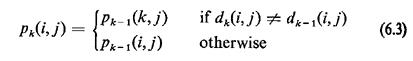
The algorithm then proceeds as follows: Shortest-Path Algorithm 2 (Algorithm 6.2)
On termination, the length, d(i, j), of the shortest path from node i to node j is given by element dn(i, j) of the final matrix D(n), while the final predecessor matrix, P(n), makes possible the tracing back of each one of the shortest paths. While the detailed example that follows should help clarify the algorithm
for the reader, its basic rationale can be quickly illustrated. Say that the
shortest path from node 4 to node 6 is the path {4, 5, 1, 7, 3, 6}. Then the
first pass (k = 1) over the algorithm will replace d(5, 7) (= Example 2
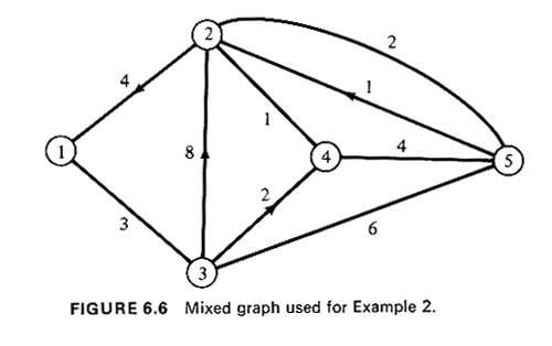
We wish to find the shortest paths between all pairs of nodes for the mixed
graph of figure 6.6. Since there are five nodes in the graph, five passes over the
algorithm will be required. The initial matrices D(0) and P(0)
and their five updated versions
are listed below. To facilitate comprehension of the example, we indicate with a " + " all
the matrix elements that have been updated from the previous pass. At each pass we also indicate
with a " * "
that row and that column (row and column k in each case) that is known a priori not to require
any changes and thus can be copied directly in the updated matrix (see Step 2 of Algorithm 6.2).
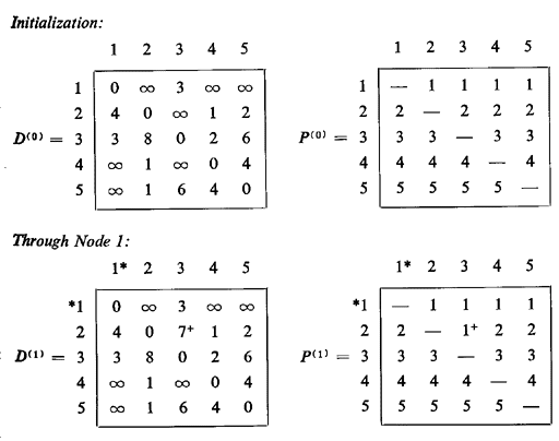
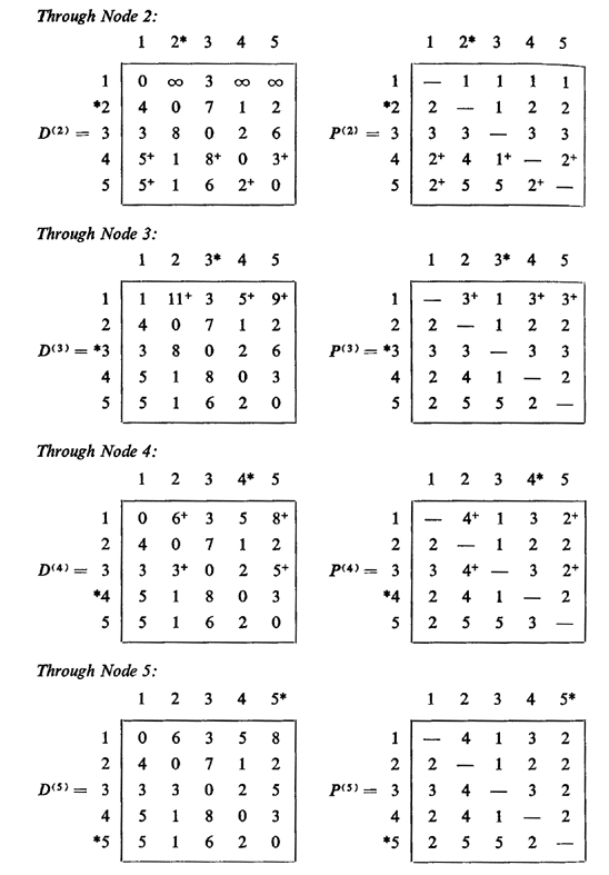
Note that on the last pass no improvements could be found for D(5) over D(4). The final matrices D(5) and P(5) indicate, for instance, that the shortest path from node 1 to node 5 has length d(1,5) = 8 units and that this shortest path is the path {1, 3, 4, 2, 5}. To identify that shortest path, we examined row 1 of the P(5) matrix. Entry p5 says that the predecessor node to 5 in the path from 1 to 5 is node 2; then, entry p5(1, 2) says that the predecessor node to 2 in the path from 1 to 2 is node 4; similarly, we backtrace the rest of the path by examining p5(1, 4) (= 3) and p5(1, 3) = 1. In general, backtracing stops when the predecessor node is the same as the initial node of the required path. For another illustration, the shortest path from node 4 to node 3 is d(4, 3) = 8 units long and the path is {4, 2, 1, 3}. The predecessor entries that must be read are, in order, p5(4, 3) = 1, p5(4, 1) = 2, and finally p5(4, 2) = 4--at which point we have "returned" to the initial node. |

 (5, 7)) by
d(5, 1) + d(l, 7) ( =
(5, 7)) by
d(5, 1) + d(l, 7) ( =