6.6.2 Discrete and Finite State Space for Probabilistic Networks

As a consequence of the conceptual and computational difficulties in obtaining shortest distances on probabilistic networks we are usually forced to make some simplifications when working with such networks. One obvious (and by far the most common) possible simplification is to use the expected link length for every link as a proxy for the true link length. This of course transforms what is actually a probabilistic network into a deterministic network with constant link lengths.

Another possible simplification which, while increasing mathematical tractability, preserves at the same time the added realism provided by the probabilistic properties of the models is the assumption that link lengths are discrete random variables that take only a finite number of values. That is, we approximate the probability distribution of random variable L(i, j), the length of the link (i, j), by writing

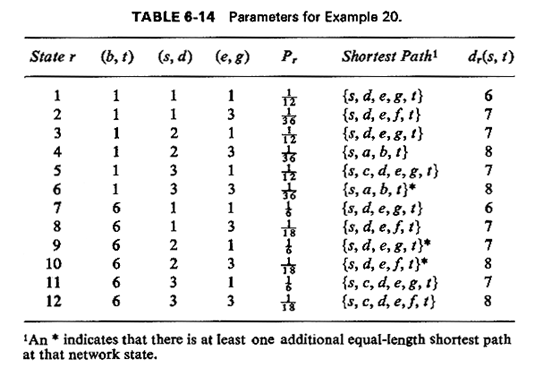
where =1. Thus, the link length can only take values ₁, ₂,...,_c. If one of these values, say _k, is infinite, we say that link (i, j) "fails with probability p_k" since, in this case, it will be impossible with probability p_k to traverse (i, j) in finite time.

The net effect of this assumption is that the network now has only a finite number, m, of states. Each state differs from the others by a change in the length of at least one link. Thus, the finest-grained sample space for the network consists of a listing of the set of all m mutually exclusive and collectively exhaustive possible network states that can be denoted as G₁, G₂, ..., G_m (to make explicit the fact that each state is a different "snapshot" of the network) with each network state having a probability of occurrence P_r, r = 1,2, ...,m.

In general, the number of states will depend on the degree of statistical dependence among the random variables
L(i, j). In the extreme case where complete statistical independence prevails, we have

where C_ij is the number of values that the length of link (i, j) [i.e., L(i, j)] can take. Similarly, the state probabilities, P_r must either be known [in the case when the L(i, j) are not mutually independent] or are easily computable (when we have statistical independence).

Let us now define:

_r(i,j) = length of link (i, j) when the network is in state G.

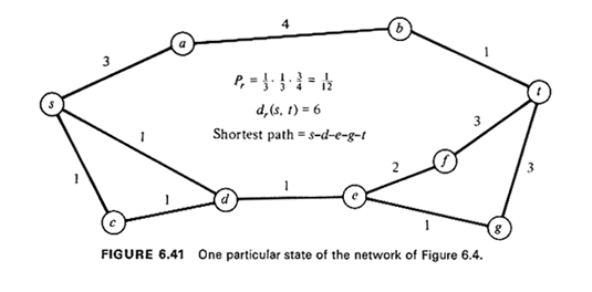
d_r(x, y) = shortest distance between points x and y when the network is in state G_r

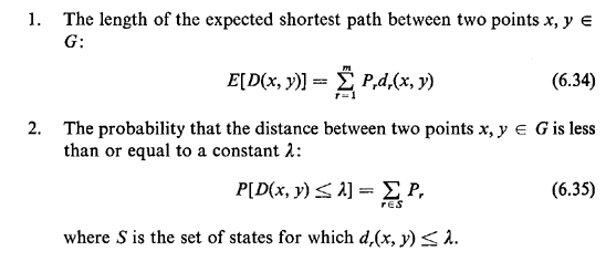
For each given state, r, the network's snapshot G_r looks exactly like a deterministic network and, therefore, using our earlier shortest-path algorithms and the known link lengths _r(i, j), we can compute the minimum distance d_r(x, y) between any two points x, y G.

In principle, then, it is possible to compute, under the assumption that there is no change of states during travel, such quantities as:

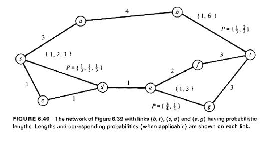
The computational effort involved may, naturally, still be formidable and depends critically on the total number m of distinct states. For instance, supposing that each link length L(i, j) takes c distinct values and assuming full statistical independence between links, we have

                            m = ce                                (6.36)

where e is the total number of links in the network. Since for a connected graph we have n - 1 e n(n - 1)/2, where n is the number of nodes in g. the number of states in the case above can be very large even for modest size networks.

On the other hand, it is very unlikely that in an urban context the link lengths will be statistically independent: traffic conditions, for example, have approximately identical time patterns throughout a city, and therefore at peak traffic times the higher values of link lengths prevail simultaneously, for all links on the network model, while the opposite is true at off-peak periods. Thus, in many cases it is possible that a few distinct states (small m) will suffice to model, at least approximately, the most common sets of travel conditions under which urban roadway networks operate. The approach that was outlined above will then prove computationally feasible under these circumstances.

Example 20: PMF for the Shortest Path Length

Consider again a graph like the one of Figure 6.40, in which all but three of the links are deterministic. The lengths of the probabilistic links L(b, t), L(s, d), and L(e, t) are assumed to take two, three, and two distinct values, respectively, with probabilities as indicated. Thus, for instance, P[L(b, t) = 6} = 2/3. We assume statistical independence between links andwish to find the distribution of the shortest distance D(s, t) between nodes s and t.

There are a total of 12 states in this case. They have been indexed with the numbers 1 through 12 (in arbitrary order) and their important parameters are tabulated in Table 6-14. Figure 6.41 shows the network in the state which has been indexed as state 1 in Table 6-14. Prom Table 6-14 it can be seen that D(s,t) takes the values 6, 7, and 8 with probability 1/4, 7/12, and 1/6, respectively.