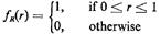
7.1.3 Generating Samples from Probability Distributions
We now turn to a discussion of how to generate sample values (i.e.,
random observations) of specific random variables. There are at least
four different ways of doing this. Throughout this section it will be
assumed that we have access to a source of "i.u.d. over [0, 1]" random
numbers. We shall denote these numbers by r (or ri, when it is necessary
to use an index). Thus, r is a sample value of the random variable R
with pdf
Inversion method. We first consider the most fundamental of the
techniques for generating sample values of random variables. It can be
applied, at least in principle, in all cases where an explicit
expression exists for the cumulative distribution function of the random
variable. Basically, the method depends on the fact that, for any random
variable Y, the cdf, Fy(y), is a non_ decreasing function with 0 </=
Fy(y) </= 1 for all values of y. This suggests a "match" of the cdf with
the random numbers, ri. Specifically, by drawing a random number r
(see Figure 7.2) and then by finding the inverse image of r on the abscissa
through
ys=Fy-1(r) (7.2)
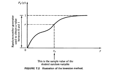
a sample value, ys, of random variable Y can be generated. To understand
why (see also Figure 7.2) observe that
P{Y</=ys} = P{R</=Fy(ys)} = Fy(ys) (7.3)
the last equality following from the fact that r is uniformly
distributed in [0,1]. The following examples illustrate the inversion
method.
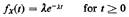
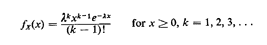
Example 1: Negative Exponential Random Variable
We have seen that the negative exponential random variable is by far the
most common model for the time between urban incidents requiring
service. It is therefore essential that we be able to generate random
sample values, ts, of the random variable X with the pdf
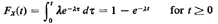
As we know, the cumulative distribution of X is
Let us then set a random number r1 (uniformly distributed between 0 and
1) equal to Fx(t). We have
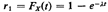
or, equivalently,
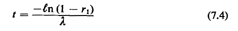
Note that (7.4) allows us to draw sample observations of X. That is,
each time we wish to draw a sample ts, all we have to do is draw a
random number r1 and use (7.4). In fact, since 1 - r1 is also a random
number uniformly distributed between 0 and 1, we might as well bypass
the subtraction and use directly the random number generated by the
computer. Thus, we finally have
 where we have used a second random number r2 as a substitute for
1 - r1.
where we have used a second random number r2 as a substitute for
1 - r1.
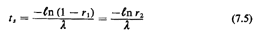
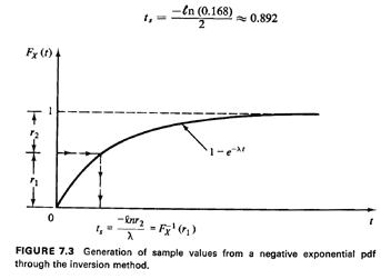
The procedure that we have used is illustrated in Figure 7.3. All we do
is draw a random number between 0 and I and then find its "inverse
image" on the t-axis by using the cdf. For a numerical example, let us
suppose that we have = 2 and that we draw the random number r = 0.168. Then
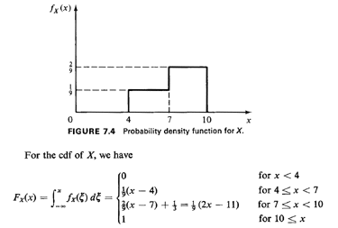
Example 2: Locations of Accidents on a Highway
Consider a 6-mile stretch of a highway, lying between the fourth- and
tenthmile points of the highway. The spatial incidence of accidents on
this 6-mile stretch is shown in Figure 7.4, which indicates that the
second half of that stretch is twice as "dangerous" as the first half.
We wish to simulate the locations of accidents on the stretch; the
locations will be denoted with the
random variable X, which is measured from the beginning of the highway
at X = 0.
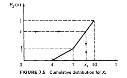
 This is plotted in Figure 7.5. In the interval of interest, [4, 101,
Fx(x) has a
breakpoint at x = 7. At that point Fx(x) =1/3. Thus, for values of a
random
number, r, which are less than 1/3, we should use r =
Fx(xs)=1/9(xs- 4)
or xs=FX-1
(r) = 9r + 4, while otherwise we should use xs =
FX-1(R)=
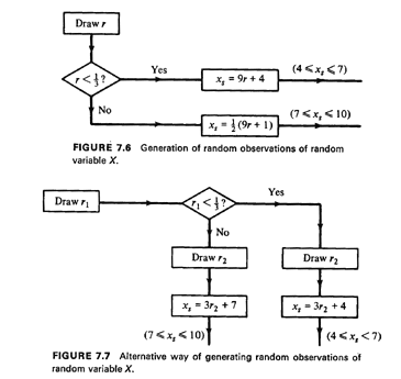
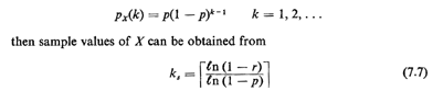
1/2(9r + 11). This procedure is illustrated in Figure 7.6. Note that the
procedure uses a single random number to generate each sample
observation, but requires some algebraic work.
We can also use an approach that requires no such work if we are willing
to generate two random numbers rather than one for each sample
observation. This alternative approach is shown by the flowchart of
Figure 7.7. Therefore, if the generation of random numbers is not
particularly time-consuming (and nowadays it is not), the alternative
approach of Figure 7.7 would probably be chosen over the one of Figure
7.6. Many variations, in terms of particular details, of either approach
may also be visualized-all leading to a satisfactory generation of
random observations of random variable X.
This is plotted in Figure 7.5. In the interval of interest, [4, 101,
Fx(x) has a
breakpoint at x = 7. At that point Fx(x) =1/3. Thus, for values of a
random
number, r, which are less than 1/3, we should use r =
Fx(xs)=1/9(xs- 4)
or xs=FX-1
(r) = 9r + 4, while otherwise we should use xs =
FX-1(R)=
1/2(9r + 11). This procedure is illustrated in Figure 7.6. Note that the
procedure uses a single random number to generate each sample
observation, but requires some algebraic work.
We can also use an approach that requires no such work if we are willing
to generate two random numbers rather than one for each sample
observation. This alternative approach is shown by the flowchart of
Figure 7.7. Therefore, if the generation of random numbers is not
particularly time-consuming (and nowadays it is not), the alternative
approach of Figure 7.7 would probably be chosen over the one of Figure
7.6. Many variations, in terms of particular details, of either approach
may also be visualized-all leading to a satisfactory generation of
random observations of random variable X.
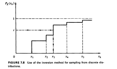
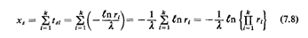
In an identical manner, we can use the inversion method to generate
amples from discrete random variables. This is shown in Figure 7.8. If
{x1, X2, X3, ... 1 are the values that the
discrete random variable X
can take and px(xk) and Px(xk) are the pmf and cdf,
respectively, of X,
the method consists of (1) drawing a random number r, and (2) finding
the smallest value xi such that
 In that case we set xs = xi (where xs denotes
the sample value of X).
Note that entire ranges of values of r now correspond to a single value
of X.
For instance, if X has a geometric pmf,
In that case we set xs = xi (where xs denotes
the sample value of X).
Note that entire ranges of values of r now correspond to a single value
of X.
For instance, if X has a geometric pmf,
 where [a] denotes "the smallest integer that is greater than or equal to
a."
where [a] denotes "the smallest integer that is greater than or equal to
a."
 Exercise 7.1 Derive (7.7).
In general, the inversion method is useful in generating sample values
of random variables whose cdf's are relatively easy to work with. Many
other random variables, whose cdf 's do not fall into this category, can
be expressed as functions of these "simple" random variables. Therefore,
the inversion method is also important as a "building block" in more
sophisticated approaches, such as those described next.
Relationships method. A second approach for generating sample
observations of a given random variable is based on taking advantage of
some known relationship between this random variable and one or more
other random variables. This method has been widely exploited in the
case of some of the best-known (and most often used in urban operations
research) pmf's and pdf's, such as the Erlang, the binomial, and the
Poisson.
Example 3: kth-Order Erlang PDF
We know that the kth-order ErIang random variable X, with pdf
 can be considered to be the sum of k independent, identically
distributed random variables, each with negative exponential pdf with
parameter
That is,
can be considered to be the sum of k independent, identically
distributed random variables, each with negative exponential pdf with
parameter
That is,
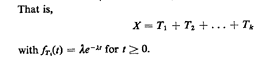 Thus, a simple way to generate random observations of X is to generate k
random observations from a negative exponential pdf by using (7.5) and
then to add these k observations to obtain a single observation of X.
That is,
Thus, a simple way to generate random observations of X is to generate k
random observations from a negative exponential pdf by using (7.5) and
then to add these k observations to obtain a single observation of X.
That is,
 The rightmost of these expressions is the most efficient one for
computational purposes. 3
The rightmost of these expressions is the most efficient one for
computational purposes. 3
Example 4: Binomial PMF
The binomial probability mass function indicates the probability of K
successes in n Bernoulli trials. To obtain sample values of K, we simply
simulate n Bernoulli trials in the computer. That is, we obtain n random
observations of a discrete random variable with probability of "success"
and of "failure"
equal to p and to 1 - p, respectively, and then count the total number
of successes in the n trials. This total number of successes is the
sample value of K.
Example 5: Simulating Poisson Events
Consider the Poisson pmf P{N(T) = k), which can be thought of as
indicating the probability of observing k events in a time interval T
when interarrival times are independent with negative exponential
distribution. To generate random observations of N(T) for any given T,
we follow the procedure shown on Figure 7.9. We keep generating
exponentially distributed time intervals
... [by using (7.5)] until the total length of time represented by the
sum of these intervals exceeds T for the first time. That is, we find j
such that
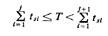 Then our sample observation of N(T) is given by ks = j.
Note how in Examples 3-5 the inversion method (for generating sample
values of negative exponential or of Bernoulli random variables) is used
as a building block (or "subroutine") in the overall procedure.
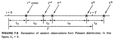
The rejection method. The rejection method is a quite ingenious approach
and is based on a geometrical probability interpretation of pdf's (cf.
Section 3.3.2). It can be used for generating sample values for any
random variable that:
| 1. | Assumes values only within a finite range.
| | 2. | Has a pdf that is bounded (i.e., does not go to infinity for any
value
of the random variable).
|
Let X be such a random variable. Let the maximum value of the pdf fx(x)
be denoted as c and let X assume values in the range [a, b] (X need not
assume all possible values in [a, b]). To generate random observations
of X through the rejection method (see Figure 7.10):
| STEP 1: | Enclose the pdf fx(x) in the smallest rectangle that fully
contains it and whose sides are parallel to the x and y axes. This is a
(b - a) x c rectangle.4
| | STEP 2: | Using two random numbers, r1 and r2, and scaling each to the
appropriate dimension of the rectangle [by multiplying one by (b - a)
and the other by c] generate a point that is uniformly distributed over
the rectangle.
| | STEP 3: | If this point is "below" the pdf, accept the x-coordinate of
the point as an appropriate sample value of X. Otherwise, reject and
return to Step 2.
|
The validity of the foregoing procedure is not intuitively obvious on a
first reading. We illustrate it first through an example and then
explain why it works.
Example 6: Locations of Accidents on a Highway, Revisited
Consider once more the problem of simulating the location of accidents
on a 6-mile stretch of highway (Example 2). For the random variable X
with pdf fx(x) (Figure 7.4), we have c 2/9, a = 4, and b = 10.
Suppose now that the pair of random numbers r1 = 0.34, r2 = 0.81 is
drawn in Step 2. These random numbers, with appropriate scaling,
identify the point (x1, y1) = [(10 - 4)(0.34) + 4, 2/9(0.81)] = (6.04,
0.18) on the x-y plane. Since at x1 = 6.04, fx(x1) 0. 11 (see Figure
7.4), the point (x1, y1) is found in Step 3 to be above fx(x) and is
rejected. No sample value of X has been obtained in this trial.
Returning to Step 2, suppose that the new pair of random numbers turns
out to be r I = 0.41, r2 = 0. 15. This results in the point (X2, y2)
(6.46,
0.033), which is below fx(x). Therefore, the sample value xs = 6.46 is
accepted.
It is easy to see in this case that the only pairs of random numbers
that will be rejected are those for which r1 ‹ 0.5 </= r2.
The reason why this method works is quite simple. The points (x, y)
obtained through the procedure of Step 2 are uniformly distributed over
the area of the rectangle, (b - a) x c. Therefore, for any point whose
x-coordinate is between x0 and x0 + dx
(see Figure 7. 10), we have
 Since the x-coordinate of the points (x, y) is chosen randomly in [a,
b], the sample observations that will be accepted will then be
distributed exactly as fx(x) In other words, were we to obtain a very
large number of sample observations, xs, and then construct a histogram
of these observations, the histogram would tend to duplicate the shape
of fx(x).
Note that the rejection method is a very general one since it makes only
the two assumptions that we have mentioned regarding the functional form
of fx(x). It is especially convenient and easy to use with pdf's which
are shaped like polygons. Its main disadvantage is that for some pdf's
it may take many rejected pairs of random numbers before an accepted
sample value is found.
Since the x-coordinate of the points (x, y) is chosen randomly in [a,
b], the sample observations that will be accepted will then be
distributed exactly as fx(x) In other words, were we to obtain a very
large number of sample observations, xs, and then construct a histogram
of these observations, the histogram would tend to duplicate the shape
of fx(x).
Note that the rejection method is a very general one since it makes only
the two assumptions that we have mentioned regarding the functional form
of fx(x). It is especially convenient and easy to use with pdf's which
are shaped like polygons. Its main disadvantage is that for some pdf's
it may take many rejected pairs of random numbers before an accepted
sample value is found.
Exercise 7.2 Show that
E[number of trials until an accepted sample value is found]
= c(b - a) (7.10)
Note: This is independent of the functional form of fx(x)!
Method of approximations. The fourth approach to generating sample
values of random variables consists simply of approximating in some way
a probability distribution by another distribution which is simpler to
simulate through one of the three earlier methods.
The classical example of this type of approach is the generation of
random observations from a Gaussian (normal) distribution.
Example 7
Generate random observations of a random variable X with a Gaussian
distribution, mean and standard deviation
Solution
No closed-form expression exists for the cumulative distribution Fx(x)
of a Gaussian random variable. Consequently, short of an approximate
numerical procedure, we cannot use the inversion method and must resort
to some other technique. One approach that can be made arbitrarily
accurate and is easy to implement is based on the Central Limit Theorem
(CLT):
Define a random variable Z as the sum of k independent random variables
uniformly distributed between 0 and 1:
Z=R1+R2+R3...+Rk+1+Rk
Now from the CLT we know that for large k, Z has approximately a
Gaussian distribution. Since for each Ri we have E[Ri] = 1/2 and
 the
mean value of Z is k/2 and its standard deviation
the
mean value of Z is k/2 and its standard deviation
 Thus, we can use
 since both sides of this equation are equal to a "normalized" Gaussian
random variable with mean 0 and standard deviation equal to 1. From
(7.11) we finally have
since both sides of this equation are equal to a "normalized" Gaussian
random variable with mean 0 and standard deviation equal to 1. From
(7.11) we finally have
 where xs is a random observation of random variable X. Generally, values
of k greater than 6 or so provide adequate approximations to the
Gaussian pdf
for values of X within two standard deviations of the mean. The most
commonly used value is k = 12, since it simplifies somewhat the
computation of (7.12). This means that we have to draw 12 random numbers
r1, r2, r12 in order to obtain a single sample
value xs of X.
where xs is a random observation of random variable X. Generally, values
of k greater than 6 or so provide adequate approximations to the
Gaussian pdf
for values of X within two standard deviations of the mean. The most
commonly used value is k = 12, since it simplifies somewhat the
computation of (7.12). This means that we have to draw 12 random numbers
r1, r2, r12 in order to obtain a single sample
value xs of X.
In general, the approximations approach is not always quite as
sophisticated as our last example might indicate. Most often, in fact,
the approach consists of simply approximating a complicated pdf (or cdf)
with, say, a piecewise linear pdf (or cdf) and then using the inversion
or the rejection method to generate random observations.
Final comment. Methods for generating samples from some of the standard
pdf's and pmf's have been the subject of much research in recent years.
Our main purpose above was to present some typical (and correct)
approaches rather than the most accurate or efficient method in each
example. For instance, excellent alternatives to (7.5) exist for
simulating negative exponential pdf's [NEUM 51], [FISH 78].
Similarly, an alternative to (7.12) for the Gaussian random variable
with mean
and variance
is the following:
| I. | Generate two random numbers r1 and r2.
| | 2. | Set:
| | 3. | Obtain samples, xs,
of the Gaussian random variable by setting

|
This method is exact and requires only two random numbers. It can be
derived from the analysis described in Example 3 of Chapter 3 (that
involved the Rayleigh distribution) and is further developed in Problem
7.2.
Many of the more advanced simulation languages/systems (e.g., GPSS,
SIMSCRIPT) provide standard internal subroutines for the generation of
samples from some of the most common pdf's and pmf's (e.g., the
Gaussian, the negative exponential, the Poisson, and the uniform): all
that a user of the language/system must do is provide the necessary
input parameters. The subroutine then automatically returns a sample
value from the specified random variable.
Review example. We review now the first three of the foregoing
approaches with an example.
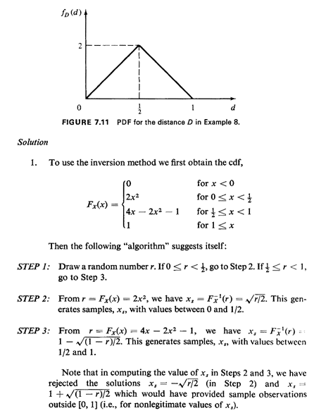
Example 8: Triangular PDF
A hospital is located at the center of a district I- by 1-mile square.
Travel is parallel to the sides of the square, and emergency patient
demands are distributed uniformly over the square. We wish to generate
sample values of the total distance between an emergency patient and the
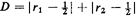
hospital. The pdf for the total distance D = D~ + D, is shown in Figure
7.11.
| 2. | If we decide to search for a relationship between random variable
X and some other random variable(s), we should be able to note
immediately that the pdf fx(x) is identical to the one that would have
resulted from the definition
 where Y1 and Y2 are independent, identically distributed random
variables with uniform distributions in [0, 1). (Readers should convince
themselves that this is so.) Therefore, a very simple method for
generating random observations of X is to use
where Y1 and Y2 are independent, identically distributed random
variables with uniform distributions in [0, 1). (Readers should convince
themselves that this is so.) Therefore, a very simple method for
generating random observations of X is to use
 where r1 and r2 are the usual random numbers obtained through the
random-number generator. This is equivalent to generating samples of the
distance traveled in the x-direction, Dx, and in the y-direction, Dy,
and adding the two.
where r1 and r2 are the usual random numbers obtained through the
random-number generator. This is equivalent to generating samples of the
distance traveled in the x-direction, Dx, and in the y-direction, Dy,
and adding the two.
| | 3. | In using the rejection method, suppose that the first pair of
random numbers drawn are r1 = 0.84 and r2 = 0.27. This results in the
point (xi, y1) = [1 · (0.84), 2· (0.27)] (0.84, 0.54) in the x-y plane.
Since at x1 = 0.84, fx(O.84) = 4(l 0.84) 0.64 (> 0.54), the sample
observation is acceptable and we set xs 0.84. Note that in this case 50
percent of the pairs will be accepted on the average.
| | 4. | "Most natural": Generate a random point
(x = r1, y = r2) in the
square and compute
|
3tsi in (7.8) denotes a sample observation of the negative
exponential random variable Ti
4 The method will actually work with any rectangle that contains this
smallest rectangle. However the probability of rejection will then be
greater than with the (b - a) x c rectangle.
|


