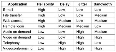
5.4 Quality of Service

The techniques we looked at in the previous sections are designed to reduce congestion and improve network performance. However, with the growth of multimedia networking, often these ad hoc measures are not enough. Serious attempts at guaranteeing quality of service through network and protocol design are needed. In the following sections we will continue our study of network performance, but now with a sharper focus on ways to provide a quality of service matched to application needs. It should be stated at the start, however, that many of these ideas are in flux and are subject to change.

5.4.1 Requirements

A stream of packets from a source to a destination is called a flow.Ina connection-oriented network, all the packets belonging to a flow follow the same route; in a connectionless network, they may follow different routes. The needs of each flow can be characterized by four primary parameters: reliability, delay, jitter, and bandwidth. Together these determine the QoS (Quality of Service) the flow requires. Several common applications and the stringency of their requirements are listed in Fig. 5-30.

The first four applications have stringent requirements on reliability. No bits may be delivered incorrectly. This goal is usually achieved by checksumming each packet and verifying the checksum at the destination. If a packet is damaged in transit, it is not acknowledged and will be retransmitted eventually. This strategy gives high reliability. The four final (audio/video) applications can tolerate errors, so no checksums are computed or verified.

File transfer applications, including e-mail and video, are not delay sensitive. If all packets are delayed uniformly by a few seconds, no harm is done. Interactive applications, such as Web surfing and remote login, are more delay sensitive. Real-time applications, such as telephony and videoconferencing have strict delay requirements. If all the words in a telephone call are each delayed by exactly 2.000 seconds, the users will find the connection unacceptable. On the other hand, playing audio or video files from a server does not require low delay.

The first three applications are not sensitive to the packets arriving with irregular time intervals between them. Remote login is somewhat sensitive to that, since characters on the screen will appear in little bursts if the connection suffers much jitter. Video and especially audio are extremely sensitive to jitter. If a user is watching a video over the network and the frames are all delayed by exactly 2.000 seconds, no harm is done. But if the transmission time varies randomly between 1 and 2 seconds, the result will be terrible. For audio, a jitter of even a few milliseconds is clearly audible.

Finally, the applications differ in their bandwidth needs, with e-mail and remote login not needing much, but video in all forms needing a great deal.

ATM networks classify flows in four broad categories with respect to their QoS demands as follows:

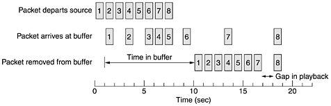
These categories are also useful for other purposes and other networks. Constant bit rate is an attempt to simulate a wire by providing a uniform bandwidth and a uniform delay. Variable bit rate occurs when video is compressed, some frames compressing more than others. Thus, sending a frame with a lot of detail in it may require sending many bits whereas sending a shot of a white wall may compress extremely well. Available bit rate is for applications, such as e-mail, that are not sensitive to delay or jitter.

5.4.2 Techniques for Achieving Good Quality of Service

Now that we know something about QoS requirements, how do we achieve them? Well, to start with, there is no magic bullet. No single technique provides efficient, dependable QoS in an optimum way. Instead, a variety of techniques have been developed, with practical solutions often combining multiple techniques. We will now examine some of the techniques system designers use to achieve QoS.

Overprovisioning

An easy solution is to provide so much router capacity, buffer space, and bandwidth that the packets just fly through easily. The trouble with this solution is that it is expensive. As time goes on and designers have a better idea of how much is enough, this technique may even become practical. To some extent, the telephone system is overprovisioned. It is rare to pick up a telephone and not get a dial tone instantly. There is simply so much capacity available there that demand can always be met.

Buffering

Flows can be buffered on the receiving side before being delivered. Buffering them does not affect the reliability or bandwidth, and increases the delay, but it smooths out the jitter. For audio and video on demand, jitter is the main problem, so this technique helps a lot.

We saw the difference between high jitter and low jitter in Fig. 5-29. In Fig. 5-31 we see a stream of packets being delivered with substantial jitter. Packet 1 is sent from the server at t = 0 sec and arrives at the client at t = 1 sec. Packet 2 undergoes more delay and takes 2 sec to arrive. As the packets arrive, they are buffered on the client machine.

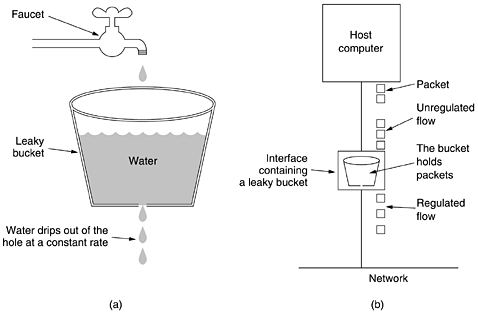
At t = 10 sec, playback begins. At this time, packets 1 through 6 have been buffered so that they can be removed from the buffer at uniform intervals for smooth play. Unfortunately, packet 8 has been delayed so much that it is not available when its play slot comes up, so playback must stop until it arrives, creating an annoying gap in the music or movie. This problem can be alleviated by delaying the starting time even more, although doing so also requires a larger buffer. Commercial Web sites that contain streaming audio or video all use players that buffer for about 10 seconds before starting to play.

Traffic Shaping

In the above example, the source outputs the packets with a uniform spacing between them, but in other cases, they may be emitted irregularly, which may cause congestion to occur in the network. Nonuniform output is common if the server is handling many streams at once, and it also allows other actions, such as fast forward and rewind, user authentication, and so on. Also, the approach we used here (buffering) is not always possible, for example, with videoconferencing. However, if something could be done to make the server (and hosts in general) transmit at a uniform rate, quality of service would be better. We will now examine a technique, traffic shaping, which smooths out the traffic on the server side, rather than on the client side.

Traffic shaping is about regulating the average rate (and burstiness) of data transmission. In contrast, the sliding window protocols we studied earlier limit the amount of data in transit at once, not the rate at which it is sent. When a connection is set up, the user and the subnet (i.e., the customer and the carrier) agree on a certain traffic pattern (i.e., shape) for that circuit. Sometimes this is called a service level agreement. As long as the customer fulfills her part of the bargain and only sends packets according to the agreed-on contract, the carrier promises to deliver them all in a timely fashion. Traffic shaping reduces congestion and thus helps the carrier live up to its promise. Such agreements are not so important for file transfers but are of great importance for real-time data, such as audio and video connections, which have stringent quality-of-service requirements.

In effect, with traffic shaping the customer says to the carrier: My transmission pattern will look like this; can you handle it? If the carrier agrees, the issue arises of how the carrier can tell if the customer is following the agreement and what to do if the customer is not. Monitoring a traffic flow is called traffic policing. Agreeing to a traffic shape and policing it afterward are easier with virtual-circuit subnets than with datagram subnets. However, even with datagram subnets, the same ideas can be applied to transport layer connections.

The Leaky Bucket Algorithm

Imagine a bucket with a small hole in the bottom, as illustrated in Fig. 5-32(a). No matter the rate at which water enters the bucket, the outflow is at a constant rate, r, when there is any water in the bucket and zero when the bucket is empty. Also, once the bucket is full, any additional water entering it spills over the sides and is lost (i.e., does not appear in the output stream under the hole).

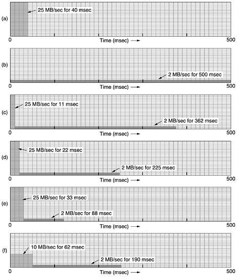
The same idea can be applied to packets, as shown in Fig. 5-32(b). Conceptually, each host is connected to the network by an interface containing a leaky bucket, that is, a finite internal queue. If a packet arrives at the queue when it is full, the packet is discarded. In other words, if one or more processes within the host try to send a packet when the maximum number is already queued, the new packet is unceremoniously discarded. This arrangement can be built into the hardware interface or simulated by the host operating system. It was first proposed by Turner (1986) and is called the leaky bucket algorithm. In fact, it is nothing other than a single-server queueing system with constant service time.

The host is allowed to put one packet per clock tick onto the network. Again, this can be enforced by the interface card or by the operating system. This mechanism turns an uneven flow of packets from the user processes inside the host into an even flow of packets onto the network, smoothing out bursts and greatly reducing the chances of congestion.

When the packets are all the same size (e.g., ATM cells), this algorithm can be used as described. However, when variable-sized packets are being used, it is often better to allow a fixed number of bytes per tick, rather than just one packet. Thus, if the rule is 1024 bytes per tick, a single 1024-byte packet can be admitted on a tick, two 512-byte packets, four 256-byte packets, and so on. If the residual byte count is too low, the next packet must wait until the next tick.

Implementing the original leaky bucket algorithm is easy. The leaky bucket consists of a finite queue. When a packet arrives, if there is room on the queue it is appended to the queue; otherwise, it is discarded. At every clock tick, one packet is transmitted (unless the queue is empty).

The byte-counting leaky bucket is implemented almost the same way. At each tick, a counter is initialized to n. If the first packet on the queue has fewer bytes than the current value of the counter, it is transmitted, and the counter is decremented by that number of bytes. Additional packets may also be sent, as long as the counter is high enough. When the counter drops below the length of the next packet on the queue, transmission stops until the next tick, at which time the residual byte count is reset and the flow can continue.

As an example of a leaky bucket, imagine that a computer can produce data at 25 million bytes/sec (200 Mbps) and that the network also runs at this speed. However, the routers can accept this data rate only for short intervals (basically, until their buffers fill up). For long intervals, they work best at rates not exceeding 2 million bytes/sec. Now suppose data comes in 1-million-byte bursts, one 40-msec burst every second. To reduce the average rate to 2 MB/sec, we could use a leaky bucket with r=2 MB/sec and a capacity, C, of 1 MB. This means that bursts of up to 1 MB can be handled without data loss and that such bursts are spread out over 500 msec, no matter how fast they come in.

In Fig. 5-33(a) we see the input to the leaky bucket running at 25 MB/sec for 40 msec. In Fig. 5-33(b) we see the output draining out at a uniform rate of 2 MB/sec for 500 msec.

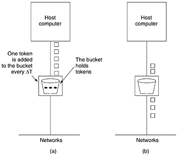
The Token Bucket Algorithm

The leaky bucket algorithm enforces a rigid output pattern at the average rate, no matter how bursty the traffic is. For many applications, it is better to allow the output to speed up somewhat when large bursts arrive, so a more flexible algorithm is needed, preferably one that never loses data. One such algorithm is the token bucket algorithm. In this algorithm, the leaky bucket holds tokens, generated by a clock at the rate of one token every DT sec. In Fig. 5-34(a) we see a bucket holding three tokens, with five packets waiting to be transmitted. For a packet to be transmitted, it must capture and destroy one token. In Fig. 5-34(b) we see that three of the five packets have gotten through, but the other two are stuck waiting for two more tokens to be generated.

The token bucket algorithm provides a different kind of traffic shaping than that of the leaky bucket algorithm. The leaky bucket algorithm does not allow idle hosts to save up permission to send large bursts later. The token bucket algorithm does allow saving, up to the maximum size of the bucket, n. This property means that bursts of up to n packets can be sent at once, allowing some burstiness in the output stream and giving faster response to sudden bursts of input.

Another difference between the two algorithms is that the token bucket algorithm throws away tokens (i.e., transmission capacity) when the bucket fills up but never discards packets. In contrast, the leaky bucket algorithm discards packets when the bucket fills up.

Here, too, a minor variant is possible, in which each token represents the right to send not one packet, but k bytes. A packet can only be transmitted if enough tokens are available to cover its length in bytes. Fractional tokens are kept for future use.

The leaky bucket and token bucket algorithms can also be used to smooth traffic between routers, as well as to regulate host output as in our examples. However, one clear difference is that a token bucket regulating a host can make the host stop sending when the rules say it must. Telling a router to stop sending while its input keeps pouring in may result in lost data.

The implementation of the basic token bucket algorithm is just a variable that counts tokens. The counter is incremented by one every DT and decremented by one whenever a packet is sent. When the counter hits zero, no packets may be sent. In the byte-count variant, the counter is incremented by k bytes every DT and decremented by the length of each packet sent.

Essentially what the token bucket does is allow bursts, but up to a regulated maximum length. Look at Fig. 5-33(c) for example. Here we have a token bucket with a capacity of 250 KB. Tokens arrive at a rate allowing output at 2 MB/sec. Assuming the token bucket is full when the 1-MB burst arrives, the bucket can drain at the full 25 MB/sec for about 11 msec. Then it has to cut back to 2 MB/sec until the entire input burst has been sent.

Calculating the length of the maximum rate burst is slightly tricky. It is not just 1 MB divided by 25 MB/sec because while the burst is being output, more tokens arrive. If we call the burst length S sec, the token bucket capacity C bytes, the token arrival rate r bytes/sec, and the maximum output rate M bytes/sec, we see that an output burst contains a maximum of C + rS bytes. We also know that the number of bytes in a maximum-speed burst of length S seconds is MS. Hence we have

We can solve this equation to get S = C/(M - r). For our parameters of C = 250 KB, M = 25 MB/sec, and r=2 MB/sec, we get a burst time of about 11 msec. Figure 5-33(d) and Fig. 5-33(e) show the token bucket for capacities of 500 KB and 750 KB, respectively.

A potential problem with the token bucket algorithm is that it allows large bursts again, even though the maximum burst interval can be regulated by careful selection of r and M. It is frequently desirable to reduce the peak rate, but without going back to the low value of the original leaky bucket.

One way to get smoother traffic is to insert a leaky bucket after the token bucket. The rate of the leaky bucket should be higher than the token bucket's r but lower than the maximum rate of the network. Figure 5-33(f) shows the output for a 500-KB token bucket followed by a 10-MB/sec leaky bucket.

Policing all these schemes can be a bit tricky. Essentially, the network has to simulate the algorithm and make sure that no more packets or bytes are being sent than are permitted. Nevertheless, these tools provide ways to shape the network traffic into more manageable forms to assist meeting quality-of-service requirements.

Resource Reservation

Being able to regulate the shape of the offered traffic is a good start to guaranteeing the quality of service. However, effectively using this information implicitly means requiring all the packets of a flow to follow the same route. Spraying them over routers at random makes it hard to guarantee anything. As a consequence, something similar to a virtual circuit has to be set up from the source to the destination, and all the packets that belong to the flow must follow this route.

Once we have a specific route for a flow, it becomes possible to reserve resources along that route to make sure the needed capacity is available. Three different kinds of resources can potentially be reserved:

The first one, bandwidth, is the most obvious. If a flow requires 1 Mbps and the outgoing line has a capacity of 2 Mbps, trying to direct three flows through that line is not going to work. Thus, reserving bandwidth means not oversubscribing any output line.

A second resource that is often in short supply is buffer space. When a packet arrives, it is usually deposited on the network interface card by the hardware itself. The router software then has to copy it to a buffer in RAM and queue that buffer for transmission on the chosen outgoing line. If no buffer is available, the packet has to be discarded since there is no place to put it. For a good quality of service, some buffers can be reserved for a specific flow so that flow does not have to compete for buffers with other flows. There will always be a buffer available when the flow needs one, up to some maximum.

Finally, CPU cycles are also a scarce resource. It takes router CPU time to process a packet, so a router can process only a certain number of packets per second. Making sure that the CPU is not overloaded is needed to ensure timely processing of each packet.

At first glance, it might appear that if it takes, say, 1 µsec to process a packet, a router can process 1 million packets/sec. This observation is not true because there will always be idle periods due to statistical fluctuations in the load. If the CPU needs every single cycle to get its work done, losing even a few cycles due to occasional idleness creates a backlog it can never get rid of.

However, even with a load slightly below the theoretical capacity, queues can build up and delays can occur. Consider a situation in which packets arrive at random with a mean arrival rate of l packets/sec. The CPU time required by each one is also random, with a mean processing capacity of µ packets/sec. Under the assumption that both the arrival and service distributions are Poisson distributions, it can be proven using queueing theory that the mean delay experienced by a packet, T, is

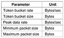
where r = l/µ is the CPU utilization. The first factor, 1/µ, is what the service time would be in the absence of competition. The second factor is the slowdown due to competition with other flows. For example, if l = 950,000 packets/sec and µ = 1,000,000 packets/sec, then r = 0.95 and the mean delay experienced by each packet will be 20 µsec instead of 1 µsec. This time accounts for both the queueing time and the service time, as can be seen when the load is very low (l/µ 0). If there are, say, 30 routers along the flow's route, queueing delay alone will account for 600 µsec of delay.

Admission Control

Now we are at the point where the incoming traffic from some flow is well shaped and can potentially follow a single route in which capacity can be reserved in advance on the routers along the path. When such a flow is offered to a router, it has to decide, based on its capacity and how many commitments it has already made for other flows, whether to admit or reject the flow.

The decision to accept or reject a flow is not a simple matter of comparing the (bandwidth, buffers, cycles) requested by the flow with the router's excess capacity in those three dimensions. It is a little more complicated than that. To start with, although some applications may know about their bandwidth requirements, few know about buffers or CPU cycles, so at the minimum, a different way is needed to describe flows. Next, some applications are far more tolerant of an occasional missed deadline than others. Finally, some applications may be willing to haggle about the flow parameters and others may not. For example, a movie viewer that normally runs at 30 frames/sec may be willing to drop back to 25 frames/sec if there is not enough free bandwidth to support 30 frames/sec. Similarly, the number of pixels per frame, audio bandwidth, and other properties may be adjustable.

Because many parties may be involved in the flow negotiation (the sender, the receiver, and all the routers along the path between them), flows must be described accurately in terms of specific parameters that can be negotiated. A set of such parameters is called a flow specification. Typically, the sender (e.g., the video server) produces a flow specification proposing the parameters it would like to use. As the specification propagates along the route, each router examines it and modifies the parameters as need be. The modifications can only reduce the flow, not increase it (e.g., a lower data rate, not a higher one). When it gets to the other end, the parameters can be established.

As an example of what can be in a flow specification, consider the example of Fig. 5-35, which is based on RFCs 2210 and 2211. It has five parameters, the first of which, the Token bucket rate, is the number of bytes per second that are put into the bucket. This is the maximum sustained rate the sender may transmit, averaged over a long time interval.

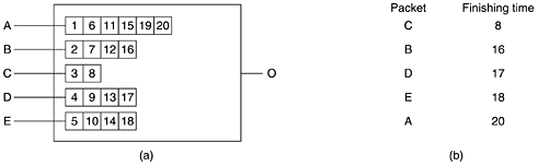
The second parameter is the size of the bucket in bytes. If, for example, the Token bucket rate is 1 Mbps and the Token bucket size is 500 KB, the bucket can fill continuously for 4 sec before it fills up (in the absence of any transmissions). Any tokens sent after that are lost.

The third parameter, the Peak data rate, is the maximum tolerated transmission rate, even for brief time intervals. The sender must never exceed this rate.

The last two parameters specify the minimum and maximum packet sizes, including the transport and network layer headers (e.g., TCP and IP). The minimum size is important because processing each packet takes some fixed time, no matter how short. A router may be prepared to handle 10,000 packets/sec of 1 KB each, but not be prepared to handle 100,000 packets/sec of 50 bytes each, even though this represents a lower data rate. The maximum packet size is important due to internal network limitations that may not be exceeded. For example, if part of the path goes over an Ethernet, the maximum packet size will be restricted to no more than 1500 bytes no matter what the rest of the network can handle.

An interesting question is how a router turns a flow specification into a set of specific resource reservations. That mapping is implementation specific and is not standardized. Suppose that a router can process 100,000 packets/sec. If it is offered a flow of 1 MB/sec with minimum and maximum packet sizes of 512 bytes, the router can calculate that it might get 2048 packets/sec from that flow. In that case, it must reserve 2% of its CPU for that flow, preferably more to avoid long queueing delays. If a router's policy is never to allocate more than 50% of its CPU (which implies a factor of two delay, and it is already 49% full, then this flow must be rejected. Similar calculations are needed for the other resources.

The tighter the flow specification, the more useful it is to the routers. If a flow specification states that it needs a Token bucket rate of 5 MB/sec but packets can vary from 50 bytes to 1500 bytes, then the packet rate will vary from about 3500 packets/sec to 105,000 packets/sec. The router may panic at the latter number and reject the flow, whereas with a minimum packet size of 1000 bytes, the 5 MB/sec flow might have been accepted.

Proportional Routing

Most routing algorithms try to find the best path for each destination and send all traffic to that destination over the best path. A different approach that has been proposed to provide a higher quality of service is to split the traffic for each destination over multiple paths. Since routers generally do not have a complete overview of network-wide traffic, the only feasible way to split traffic over multiple routes is to use locally-available information. A simple method is to divide the traffic equally or in proportion to the capacity of the outgoing links. However, more sophisticated algorithms are also available (Nelakuditi and Zhang, 2002).

Packet Scheduling

If a router is handling multiple flows, there is a danger that one flow will hog too much of its capacity and starve all the other flows. Processing packets in the order of their arrival means that an aggressive sender can capture most of the capacity of the routers its packets traverse, reducing the quality of service for others. To thwart such attempts, various packet scheduling algorithms have been devised (Bhatti and Crowcroft, 2000).

One of the first ones was the fair queueing algorithm (Nagle, 1987). The essence of the algorithm is that routers have separate queues for each output line, one for each flow. When a line becomes idle, the router scans the queues round robin, taking the first packet on the next queue. In this way, with n hosts competing for a given output line, each host gets to send one out of every n packets. Sending more packets will not improve this fraction.

Although a start, the algorithm has a problem: it gives more bandwidth to hosts that use large packets than to hosts that use small packets. Demers et al. (1990) suggested an improvement in which the round robin is done in such a way as to simulate a byte-by-byte round robin, instead of a packet-by-packet round robin. In effect, it scans the queues repeatedly, byte-for-byte, until it finds the tick on which each packet will be finished. The packets are then sorted in order of their finishing and sent in that order. The algorithm is illustrated in Fig. 5-36.

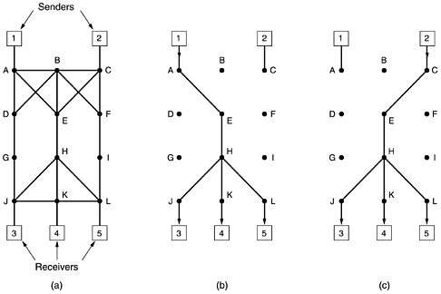
In Fig. 5-36(a) we see packets of length 2 to 6 bytes. At (virtual) clock tick 1, the first byte of the packet on line A is sent. Then goes the first byte of the packet on line B, and so on. The first packet to finish is C, after eight ticks. The sorted order is given in Fig. 5-36(b). In the absence of new arrivals, the packets will be sent in the order listed, from C to A.

One problem with this algorithm is that it gives all hosts the same priority. In many situations, it is desirable to give video servers more bandwidth than regular file servers so that they can be given two or more bytes per tick. This modified algorithm is called weighted fair queueing and is widely used. Sometimes the weight is equal to the number of flows coming out of a machine, so each process gets equal bandwidth. An efficient implementation of the algorithm is discussed in (Shreedhar and Varghese, 1995). Increasingly, the actual forwarding of packets through a router or switch is being done in hardware (Elhanany et al., 2001).

5.4.3 Integrated Services

Between 1995 and 1997, IETF put a lot of effort into devising an architecture for streaming multimedia. This work resulted in over two dozen RFCs, starting with RFCs 2205–2210. The generic name for this work is flow-based algorithms or integrated services. It was aimed at both unicast and multicast applications. An example of the former is a single user streaming a video clip from a news site. An example of the latter is a collection of digital television stations broadcasting their programs as streams of IP packets to many receivers at various locations. Below we will concentrate on multicast, since unicast is a special case of multicast.

In many multicast applications, groups can change membership dynamically, for example, as people enter a video conference and then get bored and switch to a soap opera or the croquet channel. Under these conditions, the approach of having the senders reserve bandwidth in advance does not work well, since it would require each sender to track all entries and exits of its audience. For a system designed to transmit television with millions of subscribers, it would not work at all.

RSVP—The Resource reSerVation Protocol

The main IETF protocol for the integrated services architecture is RSVP. It is described in RFC 2205 and others. This protocol is used for making the reservations; other protocols are used for sending the data. RSVP allows multiple senders to transmit to multiple groups of receivers, permits individual receivers to switch channels freely, and optimizes bandwidth use while at the same time eliminating congestion.

In its simplest form, the protocol uses multicast routing using spanning trees, as discussed earlier. Each group is assigned a group address. To send to a group, a sender puts the group's address in its packets. The standard multicast routing algorithm then builds a spanning tree covering all group members. The routing algorithm is not part of RSVP. The only difference from normal multicasting is a little extra information that is multicast to the group periodically to tell the routers along the tree to maintain certain data structures in their memories.

As an example, consider the network of Fig. 5-37(a). Hosts 1 and 2 are multicast senders, and hosts 3, 4, and 5 are multicast receivers. In this example, the senders and receivers are disjoint, but in general, the two sets may overlap. The multicast trees for hosts 1 and 2 are shown in Fig. 5-37(b) and Fig. 5-37(c), respectively.

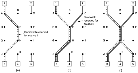
To get better reception and eliminate congestion, any of the receivers in a group can send a reservation message up the tree to the sender. The message is propagated using the reverse path forwarding algorithm discussed earlier. At each hop, the router notes the reservation and reserves the necessary bandwidth. If insufficient bandwidth is available, it reports back failure. By the time the message gets back to the source, bandwidth has been reserved all the way from the sender to the receiver making the reservation request along the spanning tree.

An example of such a reservation is shown in Fig. 5-38(a). Here host 3 has requested a channel to host 1. Once it has been established, packets can flow from 1 to 3 without congestion. Now consider what happens if host 3 next reserves a channel to the other sender, host 2, so the user can watch two television programs at once. A second path is reserved, as illustrated in Fig. 5-38(b). Note that two separate channels are needed from host 3 to router E because two independent streams are being transmitted.

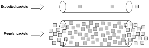
Finally, in Fig. 5-38(c), host 5 decides to watch the program being transmitted by host 1 and also makes a reservation. First, dedicated bandwidth is reserved as far as router H. However, this router sees that it already has a feed from host 1, so if the necessary bandwidth has already been reserved, it does not have to reserve any more. Note that hosts 3 and 5 might have asked for different amounts of bandwidth (e.g., 3 has a black-and-white television set, so it does not want the color information), so the capacity reserved must be large enough to satisfy the greediest receiver.

When making a reservation, a receiver can (optionally) specify one or more sources that it wants to receive from. It can also specify whether these choices are fixed for the duration of the reservation or whether the receiver wants to keep open the option of changing sources later. The routers use this information to optimize bandwidth planning. In particular, two receivers are only set up to share a path if they both agree not to change sources later on.

The reason for this strategy in the fully dynamic case is that reserved bandwidth is decoupled from the choice of source. Once a receiver has reserved bandwidth, it can switch to another source and keep that portion of the existing path that is valid for the new source. If host 2 is transmitting several video streams, for example, host 3 may switch between them at will without changing its reservation: the routers do not care what program the receiver is watching.

5.4.4 Differentiated Services

Flow-based algorithms have the potential to offer good quality of service to one or more flows because they reserve whatever resources are needed along the route. However, they also have a downside. They require an advance setup to establish each flow, something that does not scale well when there are thousands or millions of flows. Also, they maintain internal per-flow state in the routers, making them vulnerable to router crashes. Finally, the changes required to the router code are substantial and involve complex router-to-router exchanges for setting up the flows. As a consequence, few implementations of RSVP or anything like it exist yet.

For these reasons, IETF has also devised a simpler approach to quality of service, one that can be largely implemented locally in each router without advance setup and without having the whole path involved. This approach is known as class-based (as opposed to flow-based) quality of service. IETF has standardized an architecture for it, called differentiated services, which is described in RFCs 2474, 2475, and numerous others. We will now describe it.

Differentiated services (DS) can be offered by a set of routers forming an administrative domain (e.g., an ISP or a telco). The administration defines a set of service classes with corresponding forwarding rules. If a customer signs up for DS, customer packets entering the domain may carry a Type of Service field in them, with better service provided to some classes (e.g., premium service) than to others. Traffic within a class may be required to conform to some specific shape, such as a leaky bucket with some specified drain rate. An operator with a nose for business might charge extra for each premium packet transported or might allow up to N premium packets per month for a fixed additional monthly fee. Note that this scheme requires no advance setup, no resource reservation, and no time-consuming end-to-end negotiation for each flow, as with integrated services. This makes DS relatively easy to implement.

Class-based service also occurs in other industries. For example, package delivery companies often offer overnight, two-day, and three-day service. Airlines offer first class, business class, and cattle class service. Long-distance trains often have multiple service classes. Even the Paris subway has two service classes. For packets, the classes may differ in terms of delay, jitter, and probability of being discarded in the event of congestion, among other possibilities (but probably not roomier Ethernet frames).

To make the difference between flow-based quality of service and class-based quality of service clearer, consider an example: Internet telephony. With a flow-based scheme, each telephone call gets its own resources and guarantees. With a class-based scheme, all the telephone calls together get the resources reserved for the class telephony. These resources cannot be taken away by packets from the file transfer class or other classes, but no telephone call gets any private resources reserved for it alone.

Expedited Forwarding

The choice of service classes is up to each operator, but since packets are often forwarded between subnets run by different operators, IETF is working on defining network-independent service classes. The simplest class is expedited forwarding, so let us start with that one. It is described in RFC 3246.

The idea behind expedited forwarding is very simple. Two classes of service are available: regular and expedited. The vast majority of the traffic is expected to be regular, but a small fraction of the packets are expedited. The expedited packets should be able to transit the subnet as though no other packets were present. A symbolic representation of this ''two-tube'' system is given in Fig. 5-39. Note that there is still just one physical line. The two logical pipes shown in the figure represent a way to reserve bandwidth, not a second physical line.

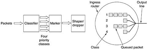
One way to implement this strategy is to program the routers to have two output queues for each outgoing line, one for expedited packets and one for regular packets. When a packet arrives, it is queued accordingly. Packet scheduling should use something like weighted fair queueing. For example, if 10% of the traffic is expedited and 90% is regular, 20% of the bandwidth could be dedicated to expedited traffic and the rest to regular traffic. Doing so would give the expedited traffic twice as much bandwidth as it needs in order to provide low delay for it. This allocation can be achieved by transmitting one expedited packet for every four regular packets (assuming the size distribution for both classes is similar). In this way, it is hoped that expedited packets see an unloaded subnet, even when there is, in fact, a heavy load.

Assured Forwarding

A somewhat more elaborate scheme for managing the service classes is called assured forwarding. It is described in RFC 2597. It specifies that there shall be four priority classes, each class having its own resources. In addition, it defines three discard probabilities for packets that are undergoing congestion: low, medium, and high. Taken together, these two factors define 12 service classes.

Figure 5-40 shows one way packets might be processed under assured forwarding. Step 1 is to classify the packets into one of the four priority classes. This step might be done on the sending host (as shown in the figure) or in the ingress (first) router. The advantage of doing classification on the sending host is that more information is available about which packets belong to which flows there.

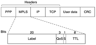
Step 2 is to mark the packets according to their class. A header field is needed for this purpose. Fortunately, an 8-bit Type of service field is available in the IP header, as we will see shortly. RFC 2597 specifies that six of these bits are to be used for the service class, leaving coding room for historical service classes and future ones.

Step 3 is to pass the packets through a shaper/dropper filter that may delay or drop some of them to shape the four streams into acceptable forms, for example, by using leaky or token buckets. If there are too many packets, some of them may be discarded here, by discard category. More elaborate schemes involving metering or feedback are also possible.

In this example, these three steps are performed on the sending host, so the output stream is now fed into the ingress router. It is worth noting that these steps may be performed by special networking software or even the operating system, to avoid having to change existing applications.

5.4.5 Label Switching and MPLS

While IETF was working out integrated services and differentiated services, several router vendors were working on better forwarding methods. This work focused on adding a label in front of each packet and doing the routing based on the label rather than on the destination address. Making the label an index into an internal table makes finding the correct output line becomes just a matter of table lookup. Using this technique, routing can be done very quickly and any necessary resources can be reserved along the path.

Of course, labeling flows this way comes perilously close to virtual circuits. X.25, ATM, frame relay, and all other networks with a virtual-circuit subnet also put a label (i.e., virtual-circuit identifier) in each packet, look it up in a table, and route based on the table entry. Despite the fact that many people in the Internet community have an intense dislike for connection-oriented networking, the idea seems to keep coming back, this time to provide fast routing and quality of service. However, there are essential differences between the way the Internet handles route construction and the way connection-oriented networks do it, so the technique is certainly not traditional circuit switching.

This ''new'' switching idea goes by various (proprietary) names, including label switching and tag switching. Eventually, IETF began to standardize the idea under the name MPLS (MultiProtocol Label Switching). We will call it MPLS below. It is described in RFC 3031 and many other RFCs.

As an aside, some people make a distinction between routing and switching. Routing is the process of looking up a destination address in a table to find where to send it. In contrast, switching uses a label taken from the packet as an index into a forwarding table. These definitions are far from universal, however.

The first problem is where to put the label. Since IP packets were not designed for virtual circuits, there is no field available for virtual-circuit numbers within the IP header. For this reason, a new MPLS header had to be added in front of the IP header. On a router-to-router line using PPP as the framing protocol, the frame format, including the PPP, MPLS, IP, and TCP headers, is as shown in Fig. 5-41. In a sense, MPLS is thus layer 2.5.

The generic MPLS header has four fields, the most important of which is the Label field, which holds the index. The QoS field indicates the class of service. The S field relates to stacking multiple labels in hierarchical networks (discussed below). If it hits 0, the packet is discarded. This feature prevents infinite looping in the case of routing instability.

Because the MPLS headers are not part of the network layer packet or the data link layer frame, MPLS is to a large extent independent of both layers. Among other things, this property means it is possible to build MPLS switches that can forward both IP packets and ATM cells, depending on what shows up. This feature is where the ''multiprotocol'' in the name MPLS came from.

When an MPLS-enhanced packet (or cell) arrives at an MPLS-capable router, the label is used as an index into a table to determine the outgoing line to use and also the new label to use. This label swapping is used in all virtual-circuit subnets because labels have only local significance and two different routers can feed unrelated packets with the same label into another router for transmission on the same outgoing line. To be distinguishable at the other end, labels have to be remapped at every hop. We saw this mechanism in action in Fig. 5-3. MPLS uses the same technique.

One difference from traditional virtual circuits is the level of aggregation. It is certainly possible for each flow to have its own set of labels through the subnet. However, it is more common for routers to group multiple flows that end at a particular router or LAN and use a single label for them. The flows that are grouped together under a single label are said to belong to the same FEC (Forwarding Equivalence Class). This class covers not only where the packets are going, but also their service class (in the differentiated services sense) because all their packets are treated the same way for forwarding purposes.

With traditional virtual-circuit routing, it is not possible to group several distinct paths with different end points onto the same virtual-circuit identifier because there would be no way to distinguish them at the final destination. With MPLS, the packets still contain their final destination address, in addition to the label, so that at the end of the labeled route the label header can be removed and forwarding can continue the usual way, using the network layer destination address.

One major difference between MPLS and conventional VC designs is how the forwarding table is constructed. In traditional virtual-circuit networks, when a user wants to establish a connection, a setup packet is launched into the network to create the path and make the forwarding table entries. MPLS does not work that way because there is no setup phase for each connection (because that would break too much existing Internet software).

Instead, there are two ways for the forwarding table entries to be created. In the data-driven approach, when a packet arrives, the first router it hits contacts the router downstream where the packet has to go and asks it to generate a label for the flow. This method is applied recursively. Effectively, this is on-demand virtual-circuit creation.

The protocols that do this spreading are very careful to avoid loops. They often use a technique called colored threads. The backward propagation of an FEC can be compared to pulling a uniquely colored thread back into the subnet. If a router ever sees a color it already has, it knows there is a loop and takes remedial action. The data-driven approach is primarily used on networks in which the underlying transport is ATM (such as much of the telephone system).

The other way, used on networks not based on ATM, is the control-driven approach. It has several variants. One of these works like this. When a router is booted, it checks to see for which routes it is the final destination (e.g., which hosts are on its LAN). It then creates one or more FECs for them, allocates a label for each one, and passes the labels to its neighbors. They, in turn, enter the labels in their forwarding tables and send new labels to their neighbors, until all the routers have acquired the path. Resources can also be reserved as the path is constructed to guarantee an appropriate quality of service.

MPLS can operate at multiple levels at once. At the highest level, each carrier can be regarded as a kind of metarouter, with there being a path through the metarouters from source to destination. This path can use MPLS. However, within each carrier's network, MPLS can also be used, leading to a second level of labeling. In fact, a packet may carry an entire stack of labels with it. The S bit in Fig. 5-41 allows a router removing a label to know if there are any additional labels left. It is set to 1 for the bottom label and 0 for all the other labels. In practice, this facility is mostly used to implement virtual private networks and recursive tunnels.

Although the basic ideas behind MPLS are straightforward, the details are extremely complicated, with many variations and optimizations, so we will not pursue this topic further. For more information, see (Davie and Rekhter, 2000; Lin et al., 2002; Pepelnjak and Guichard, 2001; and Wang, 2001).