Example-Balancing Scales

Consider the set of scales  shown in Figure . Suppose we are given a collection of n weights, , and we are required to place all of the weights onto the scales so that they are balanced.

  
Figure: A set of scales.

The problem can be expressed mathematically as follows: Let represent the pan in which weight is placed such that

The scales are balanced when the sum of the weights in the left pan equals the sum of the weights in the right pan,

Given an arbitrary set of n weights, there is no guarantee that a solution to the problem exists. A solution always exists if, instead of balancing the scales, the goal is to minimize the difference between between the total weights in the left and right pans. Thus, given , our objective is to minimize where

subject to the constraint that all the weights are placed on the scales.

Given a set of scales and collection of weights, we might solve the problem by trial-and-error: Place all the weights onto the pans one-by-one. If the scales balance, a solution has been found. If not, remove some number of the weights and place them back on the scales in some other combination. In effect, we search for a solution to the problem by first trying one solution and then backing-up to try another.

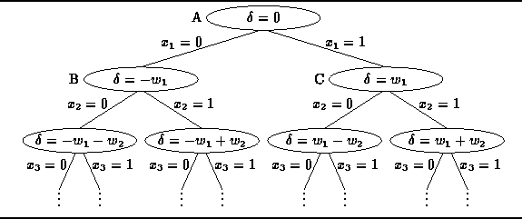
Figure  shows the solution space  for the scales balancing problem. In this case the solution space takes the form of a tree: Each node of the tree represents a partial solution to the problem. At the root (node A) no weights have been placed yet and the scales are balanced. Let be the difference between the the sum of the weights currently placed in the left and right pans. Therefore, at node A.

  
Figure: Solution space for the scales balancing problem.

Node B represents the situation in which weight has been placed in the left pan. The difference between the pans is . Conversely, node C represents the situation in which the weight has been placed in the right pan. In this case . The complete solution tree has depth n and leaves. Clearly, the solution is the leaf node having the smallest value.

In this case (as in many others) the solution space is a tree. In order to find the best solution a backtracking algorithm visits all the nodes in the solution space. That is, it does a tree traversal . Section  presents the two most important tree traversals--depth-first  and breadth-first . Both kinds can be used to implement a backtracking algorithm.

Copyright © 1998 by Bruno R. Preiss, P.Eng. All rights reserved.