11.4 Mergesort

  Sorting is a common and important problem in computing. Given a   sequence of N data elements, we are required to generate an   ordered sequence that contains the same elements. Here, we present a   parallel version of the well-known mergesort algorithm. The   algorithm assumes that the sequence to be sorted is distributed and so generates a distributed sorted sequence. For simplicity, we assume that N is an integer multiple of P , that the N data are distributed evenly among P tasks, and that is an integer power of two. Relaxing these assumptions does not change the essential character of the algorithm but would complicate the presentation.

 
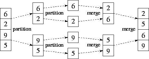
Figure 11.4: Mergesort, used here to sort the sequence [6,2,9,5]. The two partition phases each split the input sequence; the two merge phases each combine two sorted subsequences generated in a previous phase. 

The sequential mergesort algorithm is as follows; its execution is illustrated in Figure 11.4.  

1. If the input sequence has fewer than two elements, return.
2. Partition the input sequence into two halves.
3. Sort the two subsequences using the same algorithm.
4. Merge the two sorted subsequences to form the output sequence.

The merge operation employed in step (4) combines two sorted subsequences to produce a single sorted sequence. It repeatedly compares the heads of the two subsequences and outputs the lesser value until no elements remain. Mergesort requires time to sort N elements, which is the best that can be achieved (modulo constant factors) unless data are known to have special properties such as a known distribution or degeneracy.

  We first describe two algorithms required in the implementation of parallel mergesort: compare-exchange and parallel merge.

Compare-Exchange.

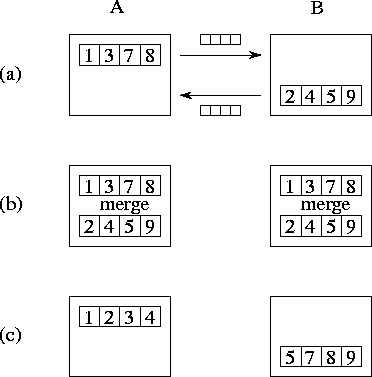
  A compare-exchange operation merges two sorted sequences of length M , contained in tasks A and B . Upon completion of the operation, both tasks have M data, and all elements in task A are less than or equal to all elements in task B . As illustrated in Figure 11.5, each task sends its data to the other task. Task A identifies the M lowest elements and discards the remainder; this process requires at least M/2 and at most M comparisons. Similarly, task B identifies the M highest elements.

 
Figure 11.5: The compare-exchange algorithm, with M=4 . (a) Tasks A and B exchange their sorted subsequences. (b) They perform a merge operation to identify the lowest and highest M elements, respectively. (c) Other elements are discarded, leaving a single sorted sequence partitioned over the two tasks. 

Notice that a task may not need all M of its neighbor's data in order to identify the M lowest (or highest) values. On average, only M/2 values are required. Hence, it may be more efficient in some situations to require the consumer to request data explicitly. This approach results in more messages that contain a total of less than M data, and can at most halve the amount of data transferred.

 
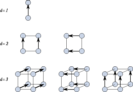
Figure 11.6: The parallel merge operation, performed in hypercubes of dimension one, two, and three. In a hypercube of dimension d , each task performs d compare-exchange operations. Arrows point from the ``high'' to the ``low'' task in each exchange. 

Parallel Merge.

A parallel merge algorithm performs a merge operation on two sorted sequences of length , each distributed over tasks, to produce a single sorted sequence of length distributed over tasks. As illustrated in Figure 11.6, this is achieved by using the hypercube communication template. Each of the tasks engages in d+1 compare-exchange steps, one with each neighbor. In effect, each node executes Algorithm 11.1, applying the following operator at each step.

 
		 if ( myid AND  > 0 ) then

				 state = compare_exchange_high(state,message)

		 else

				 state = compare_exchange_low(state,message)

		 endif

In this code fragment, AND is a bitwise logical and operator, used to determine whether the task is ``high'' or ``low'' in a particular exchange; myid and i are as in Algorithm 11.1.

Mergesort.

We next describe the parallel mergesort algorithm proper. Each task in the computation executes the following logic.

    procedure parallel_mergesort(myid, d, data, newdata)
    begin
      data = sequential_mergesort(data)
      for dim = 1 to d
        data = parallel_merge(myid, dim, data)
      endfor
      newdata = data
    end

First, each task sorts its local sequence using sequential mergesort. Second, and again using the hypercube communication structure, each of the tasks executes the parallel merge algorithm d times, for subcubes of dimension 1.. d . The i th parallel merge takes two sequences, each distributed over tasks, and generates a sorted sequence distributed over tasks. After d such merges, we have a single sorted list distributed over tasks.

Performance

  Parallel mergesort uses the hypercube communication template at multiple levels. We review these uses and develop a performance model. We assume N data distributed over tasks (that is, ), with N an integer multiple of P . Hence, the total number of compare-exchanges is

Because each compare-exchange requires one message containing N/P data, the per-processor communication cost is

The computation costs comprise the initial intraprocessor sort and the comparisons performed during the interprocessor communication phase. The former involves a total of comparisons, while the latter requires at most comparisons, thereby giving computation costs summed over P processors of

Because the algorithm is perfectly balanced, we can assume that idle time is negligible. Thus, we obtain the following model for parallel execution time: