Software Implementation in Matlab

In Matlab or Octave, this type of filter can be implemented using the filter function. For example, the following matlab^4.1 code computes the output signal y given the input signal x for a specific example comb filter:

g1 = (0.5)^3;        % Some specific coefficients
g2 = (0.9)^5;
B = [1 0 0 g1];      % Feedforward coefficients, M1=3
A = [1 0 0 0 0 g2];  % Feedback coefficients, M2=5
N = 1000;            % Number of signal samples
x = rand(N,1);       % Random test input signal
y = filter(B,A,x);   % Matlab and Octave compatible

The example coefficients, $g1 = 0.5^3 = 0.125$ and $g2 = 0.9^5 = 0.59049$, are chosen to place all filter zeros at radius $0.5$ and all filter poles at radius $0.9$ in the complex $z$ plane (as we shall see below).

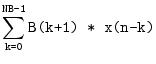
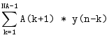
The matlab filter function carries out the following computation for each element of the y array:

$$\texttt{y(n)} = \sum_{\texttt{k=0}}^\texttt{NB-1} \texttt{B(k+1) * x(n-k)}$$ (4.2)

$$- \sum_{\texttt{k=1}}^\texttt{NA-1} \texttt{A(k+1) * y(n-k)} \protect$$ (4.3)

for $\texttt{n}=1,2,\dots,\texttt{N}$, where NA = length(A) and NB = length(B). Note that the indices of x and y can go negative in this expression. By default, such terms are replaced by zero. However, the filter function has an optional fourth argument for specifying the initial state of the filter, which includes past input and past output samples seen by the filter. This argument is used to forward the filter's state across successive blocks of data:

[y1,state] = filter(B,A,x1);       % filter 1st block x1
[y2,state] = filter(B,A,x2,state); % filter 2nd block x2
...