It is easy to check that the bilinear transform gives a one-to-one,
order-preserving, conformal map [57] between the
analog frequency axis
![]() and the digital frequency axis
and the digital frequency axis
![]() , where
, where ![]() is the sampling interval. Therefore, the
amplitude response takes on exactly the same values over both axes,
with the only defect being a
frequency warping such
that equal increments along the unit circle in the
is the sampling interval. Therefore, the
amplitude response takes on exactly the same values over both axes,
with the only defect being a
frequency warping such
that equal increments along the unit circle in the ![]() plane
correspond to larger and larger bandwidths along the
plane
correspond to larger and larger bandwidths along the ![]() axis in
the
axis in
the ![]() plane. Some kind of frequency warping is obviously
unavoidable in any one-to-one map because the analog frequency axis is
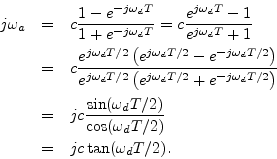
infinite while the digital frequency axis is finite. The relation
between the analog and digital frequency axes may be derived
immediately from Eq. (G.9) as
plane. Some kind of frequency warping is obviously
unavoidable in any one-to-one map because the analog frequency axis is
infinite while the digital frequency axis is finite. The relation
between the analog and digital frequency axes may be derived
immediately from Eq. (G.9) as
Given an analog cut-off frequency
![]() , to obtain the
same cut-off frequency in the digital filter, we set
, to obtain the
same cut-off frequency in the digital filter, we set