|
|
Languages like D, DR, and DV are pure-functional languages. Once we add any kind of side-effect to a language it is not pure-functional anymore. Side-effects are non-local, meaning they can affect other parts of the program. As an example, consider the following Caml code.
This expression evaluates to 10. Even though x was defined as a reference to 9 when f was declared, the last line sets x to be a reference to 5, and during the application of f, x is reassigned to be a reference to (5 + 5), making it 10 when it is finally dereferenced in the last line. Clearly, the use of side effects makes a program much more difficult to analyze, since it is not as declarative a functional program. When looking at programs with side-effects, one must examine the entire body of code to see which side-effects influence the outcome of which expressions. Therefore, is it a good programming moral to use side-effects sparingly, and only when needed.
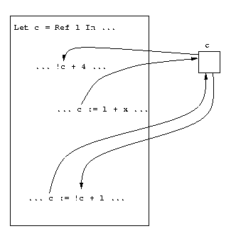
Let us begin by informally discussing the semantics of references. In essence, when a reference is created in a program, a cell is created that contains the specified value, and the reference itself is a pointer to that cell. A good metaphor for these reference cells is to think of each one as a junction box. Then, each assignment is a path into the junction, and each read, or dereference, is a path going out of the junction. The reference cell, or junction, sits to the side of the program, and allows distant parts of the program to communicate with one another. This “distant communication” can be a useful programming paradigm, but again it should be used sparingly. Figure 4.1 illustrates this metaphor.
In the world of C++ and Java, non-const (or non-final) global variables are the most notorious form of reference. While globals make it easy to do certain tasks, they generally make programs difficult to debug, since they can be altered anywhere in the code.
Adding state to our language involves making significant modifications to the pure-functional languages that we’ve looked at so far. Therefore, we will spend a bit of time developing a solid operational semantics for our state-based language before looking at the interpreter. We will define a language DS: D with state.
The most significant departure from the pure-functional operational semantics we have looked at so far is that the evaluation relation e ==> v is not sufficient to capture the semantics of a state-based language. The evaluation of an expression can now produce side-effects, and our ==> rule needs to incorporate this somehow. Specifically, we will need to have someplace to record all these side-effects: a store. In C, a store is a stack and a heap, and memory locations are referenced by their addresses. When we are writing our interpreter, we will only have access to the heap, so we will need to create an abstract store in which to record side-effects.
Cell names are an abstract representation of a memory location. A store is therefore an abstraction of a runtime heap. The C heap is a low-level realization of a store where the cell names are simply numerical memory addresses. A store is also known as a dictionary from a data-structures perspective. We write Dom(S) to refer the domain of this finite map, that is, the set of all cells that it maps.
Let us begin by extending the concrete syntax of D to include DS expressions. The additions are as follows.
We need cell names because Ref 5 needs to evaluate to a location, c, in the store. Because cell names refer to locations in the heap, and the heap is initially empty, programs have no cell names when the begin execution.
Although not part of the DS syntax, we will need a notation to represent operations on the store. We write S{c |-> v} to indicate the store S extended or modified to contain the mapping c |-> v. We write S(c) to denote the value of cell c in store S.
Now that we have developed the notion of a store, we can define a satisfactory evaluation relation for DS. Evaluation is written as follows.
<e,S0> ==> <v,S>,
where at the start of computation, S0 is initially empty, and where S is the final store when computation terminates. In the process of evaluation, cells, c, will begin to appear in the program syntax, as references to memory locations. Cells are values since they do not need to be evaluated, so the value space of DS also includes cells, c.
Finally, we are ready to write the evaluation rules for DS. We will need to modify all of the D rules with the store in mind (recall that our evaluation rule is now <e,S0> ==> <v,S>, not simply e ==> v). We do this by threading the store along the flow of control. Doing this introduces a great deal more dependency between the rules, even the ones that do not directly manipulate the store. We will rewrite the function application rule for DS to illustrate the types of changes that are needed in the other rules.
| (Function Application) |
|
Note how the store here is threaded through the different evaluations, showing how changes in the store in one place propagate to the store in other places, and in a fixed order that reflects the indented evaluation order. The rules for our new memory operations are as follows.
| (Reference Creation) |
| |||
| (Dereference) |
| |||
| (Assignment) |
|
These rules can be tricky to evaluate because the store needs to be kept up to date at all points in the evaluation. Let us look at a few example expressions to get a feel for how this works.
|
Just as we had to modify the evaluation relation in our DS operational semantics to support state, writing a DS interpreter will also require some additional work. There are two obvious approaches to take, and we will treat them both below. The first approach involves mimicking the operational semantics and defining evaluation on an expression and a store together. This approach yields a functional interpreter in which eval(e,S0) for expression e and initial state S0 returns the tuple (v,S), where v is the resulting value and S is the final state.
The second and more efficient design involves keeping track of state in a global, mutable dictionary structure. This is generally how real implementations work. This approach results in more familiar evaluation semantics, namely eval e returns v. Obviously such an interpreter is no longer functional, but rather, imperative. We would like such an interpreter to faithfully implement the operational semantics of DS, and thus we would ideally want a theorem that states that this approach is equivalent to the first approach. Proving such a theorem would be difficult, however, mainly because our proof would rely on the operational semantics of Caml, or whatever implementation language we chose. We will therefore take it on good faith that the two approaches are indeed equivalent.
The Functional Interpreter The functional interpreter implements a stateful language in a functional way. It threads the state through the evaluation, just as we did when we defined our operational semantics. Imperative style programming can be “hacked” into a functional style by threading the state along, and there are regular methods for threading state through any functional programs, namely monads. The threading approach to modeling state functionally was first employed by Strachey in the late 1960’s [22]. Note that an operational semantics is always pure functional, since mathematics is always purely functional.
To implement the functional interpreter, we model the store using a finite mapping of integer keys to values. The skeleton of the implementation is presented below.
The Imperative Interpreter The stateful, imperative DS interpreter is more efficient than its functional counterpart, because no threading is needed. In the imperative interpreter, we represent the store as a dictionary structure (similar to Java’s HashMap class or the C++ STL map template). The eval function needs no extra store parameter, provided that it has a reference to the global dictionary. Non-store-related rules such as Plus and Minus are completely ignorant of the store. Only the direct store evaluation rules, Ref, Set, and Get actually extend, update, or query the store. A good evaluator would also periodically garbage collect, or remove unneeded store elements. Garbage collection is discussed briefly in Section 4.1.4. The implementation of the stateful interpreter is left as an exercise to the reader.
Now that we have a mutable store, our code has properties beyond the value that is returned, namely, side-effects. Operators such as sequencing (;), and While- and For loops now become relevant. These syntactic concepts are easily defined as macros, so we will not add them to the official DS syntax. The macro definitions are as follows.
| e1; e2 = (Function x -> e2) e1 |
| While e Do e' = Let Rec f x = If e Then f e' Else 0 In f 0 |
Exercise 4.1. Why are sequencing and loop operations irrelevant in pure functional languages like D?
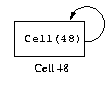
An interesting phenomenon is possible with stateful languages. It is possible to make a cyclical store, that is, a cell whose contents are a pointer to itself. Creating a cyclic store is quite easy:
Let x = Ref 0 in x := x
This is the simplest possible store cycle, where a cell directly points to itself. This type of store is illustrated in Figure 4.2.
Exercise 4.2. In the above example, what does !!!!!!!!x return? Can a store cycle like the one above be written in Caml? Why or why not? (Hint: What is the type of such an expression?)
A more subtle form of a store cycle is when a function is placed in the cell, and the body of the function refers to that cell. Consider the following example.
| Let c = Ref 0 In |
| c := (Function x -> If x = 0 Then 0 Else 1 + !c(x-1)); |
| !c(10) |
Cell c contains a function, which, in turn, refers to c. In other words, the function has a reference to itself, and can apply itself, giving us recursion. This form of recursion is known as tying the knot, and is the method used by most compilers to implement recursion. A similar technique is used to make objects self-aware, although C++ explicitly passes self, and is more like the Y -combinator.
Exercise 4.3. Tying the knot be written in Caml, but not directly as above. How must the reference be declared for this to work? Why can we create this sort of cyclic store, but not the sort described in Exercise 4.2?
|
Languages like C++, Java, and Scheme have a different form for expressing mutation. There is no need for an explicit dereference (!) operator to get the value of a cell. This form of mutation is more difficult to capture in an interpreter, because variables mean something different depending on whether they are on the left or right side of an assignment operator. An l-value occurs on the left side of the assignment, and represents a memory location. An r-value to the right of an assignment, or elsewhere in the code, and represents an actual value.
Consider the C/C++/Java assignment statement x = x + 1. The x on the left of the assignment is an l-value, and the x in x + 1 is an r-value. In Caml, we would write a similar expression as x := !x + 1. Thus, Caml is explicit in which is being referred to, the cell or the value. For a Java l-value, the cell is needed to perform the store operation, and for a Java r-value, the value of the cell is needed, which is why, in Caml, we must write !x.
l-values and r-values are distinct. Some expressions may be both l-values and r-values, such as x and x[3]. Other values may only be r-values, such as 5, (0 == 1), and sin(3.14159). Therefore, l-values and r-values are expressed differently in the language grammar, specifically, l-values are a subset of r-values. There are some shortcomings to such languages. For example, in Caml we can say f(3) := 1, which assigns the value 1 to the cell returned by the function f. Expressions of this sort are invalid in Java, because f(3) is not an l-value. We could revise the DS grammar to use this more restrictive notion, where l-values must only be variables, in the following way:
For the variable on the left side of the assignment, we would need the address, and not the contents, of the variable.
A final issue with the standard notion of state in C and C++ is the problem of uninitialized variables. Because variables are not required to be initialized, runtime errors due to these uninitialized variables are possible. Note that the Ref syntax of DS and Caml requires that the variable be explicitly initialized as part of its declaration.
Memory that is allocated may also, at some point, be freed. In C and C++, this is done explicitly with free() and delete() respectively. However, Java, Caml, Smalltalk, Scheme, and Lisp, to name a few, support the automated freeing of unused memory through a garbage collector.
Garbage collection is a large area of research (see [23] for a survey), but we will briefly sketch out what an implementation looks like.
First, something triggers the garbage collector. Generally, the trigger is that the store is getting too full. In Java, the garbage collector may be explicitly invoked by the method System.gc(). When the garbage collector is invoked, evaluation is suspended until the garbage collector has completed. The garbage collector proceeds to scan through the current computation to find cells that are directly used. The set of these cells is known as the root set. Good places to look for roots are on the evaluation stack and in global variable locations.
Once the root set is established, the garbage collector marks all cells not in the root set as initially free. Then, it recursively traverses the memory graph starting at the root set, and marks cells that are reachable from the root set as not free, thus at the end of the traversal, all cells that are in a different connected component from any of the cells in the root set are marked not free, and these cells may be reused. There are many different ways to reuse memory, but we will not go into detail here.
Now that we have discussed stateful languages, we are going to briefly touch on some efficiency issues with the way we have been defining interpreters. We will focus on eliminating explicit substitutions in function application.
A “low-level” interpreter would never duplicate the function argument for each variable usage. The problem with doing so is that it can severely increase the size of the data that must be maintained by the interpreter. Consider an expression in the following form.
(Function x -> x x x) (whopping expr)
This expression is evaluated by computing
(whopping expr)(whopping expr)(whopping expr),
tripling the size of the data.
In order to solve this problem, we define an explicit environment interpreter. In an explicit environment interpreter, instead of doing direct variable substitution, we keep track of each variable’s value in a runtime environment. The runtime environment is simply a mapping of variables to values. We write environments as {x1 |-> v1,x2 |-> v2}, to mean that variable x1 maps to value v1 and variable x2 maps to value v2.
Now, to compute
(Function x -> x x x)(whopping expr)
the interpreter computes (x x x) in the environment {x |-> whopping expr}.
Technically, even the simple substituting interpreters we’ve looked at don’t really make three copies of the data. Rather, they maintain a single copy of the data and three pointers to it. This is because immutable data can always be passed by reference since it never changes. However, in a compiler the code can’t be copied around like this, so a scheme like the one presented above is necessary.
There is a possibility for some anomalies with this approach, however. Specifically, there is a problem when a function is returned as the result of another function application, and the returned function has local variables in it. Consider the following example.
| f = Function x -> If x = 0 Then |
| Function y -> y |
| Else Function y -> x + y |
When f (3) is computed, the environment binds x to 3 while the body is computed, so the result returned is
Function y -> x + y,
but it would be a mistake to simply return this as the correct value, because we would lose the fact that x was bound to 3. The solution is that when a function value is returned, the closure of that function is returned.
Definition 4.2 (Closure). A closure is a function along with an environment, such that all free values in the function body are bound to values in the environment.
For the case above, the correct value to return is the closure
(Function y -> x + y,{x |-> 3})
Theorem 4.1. A substitution-based interpreter and an explicit environment interpreter for D are equivalent: all D programs either terminate on both interpreters or compute forever on both interpreters.
This closure view of function values is critical when writing a compiler, since compiler’s should not be doing substitutions of code on the fly. Compilers are discussed in Chapter 7.
We can now define the DSR language. DSR is the call-by-value language that included the basic features of D, and is extended to include records (DR), and state (DS).
In Section 4.4 and Chapters 5 and 6, we will study the language features missing from DSR, namely objects, exceptions, and types. In Chapter 7, we will discuss translations for DSR, but will not include these other language features. The abstract syntax type for DSR is as follows.
In the next two sections we will look at some nontrivial “real-world” DSR programs to illustrate the power we can get from this simple language. We begin by considering a function to calculate the factorial function, and conclude the chapter by examining an implementation of the merge sort algorithm.
The factorial function is fairly easy to represent using DSR. The main point of interest here is the encoding of multiplication using a curried Let Rec definition. This example assumes a positive integer input.
Writing a merge sort in DSR is a fairly comprehensive example. One of the biggest challenges is encoding integer comparisons, i.e. <, >, etc. Let’s discuss how this is accomplished before looking at the code.
First of all, given that we already have an equality test, =, encoding the <= operation basically gives us the other standard comparison operations for free. Assuming that we have a lesseq function, the other operations can be trivially encoded as follows.
Therefore it suffices to encode lesseq. But how can we do this using only the regular DSR operators? The basic idea is as follows. To test if x is less than or equal to y we compute a z such that x + z = y. If z is nonnegative, we know that x is less than or equal to y. If z is negative, we know that x is greater than y.
At first glance, we seem to have a “chicken and egg” problem here. How can we tell if z is negative if we have no comparison operator. And how do we actually compute z to begin with? One idea would be to start with z = 0 and loop, incrementing z by 1 at every step, and it testing if x + z = y. If we find a z, we stop. We know that z is positive, and we conclude that x is less than or equal to y. If we don’t find a z, we start at z = -1 and perform a similar loop, decrementing z by 1 every step. If we find a proper value of z this way, we conclude that x is greater then y.
The flaw in the above scheme should be obvious: if x > y, the first loop will never terminate. Indeed we would need to run both loops in parallel for this idea to work! Obviously DSR doesn’t allow for parallel computation, but there is a solution along these lines. We can interleave the values of z that are tested by the two loops. That is, we can try the values {0,-1,1,-2,2,-3,...}.
The great thing about this approach is that every other value of z is negative, and we can simply pass along a boolean value to represent the sign of z. If z is nonnegative, the next iteration of the loop inverts it and subtracts 1. If z is negative, the next iteration simply inverts it. Note that we can invert the sign of an number x in DSR by simply writing 0 - x. Now, armed with our ideas about lesseq, let us start writing our merge sort.
Until now, expressions have been evaluated by marching through the evaluation rules one at a time. To perform addition, the left and right operands were evaluated to values, after which the addition expression itself was evaluated to a value. This addition expression may have been part of a larger expression, which could then itself have been evaluated to a value, etc.
In this section, we will discuss explicit control operations, concentrating on exceptions. Explicit control operations are operations that explicitly alter the control of the evaluation process. Even simple languages have control operations. A common example is the return statement in C++ and Java.
In D, the value of the function is whatever its entire body evaluates to. If, in the middle of some complex conditional loop expression, we have the final result of the computation, it is still necessary to complete the execution of the function. A return statement gets around this problem by immediately returning from the function and aborting the rest of the function computation.
Another common control operation is the loop exit operation, or break in C++ or Java. break is similar to return, except that it exits the current loop instead of the entire function.
These types of control operations are interesting, but in this section, we will concentrate more on two more powerful control operations, namely exceptions and exception handlers. The reader should already be familiar with the basics of exceptions from working with the Caml exception mechanism.
There are some other control operations that we will not discuss, such as the call/cc, shift/reset, and control/prompt operators.
We will avoid the goto operator in this section, except for the following brief discussion. goto basically jumps to a labeled position in a function. The main problem with goto is that it is too raw. The paradigm of jumping around between labels is not all that useful in the context of functions. It is also inherently dangerous, as one may inadvertently jump into the middle of a function that is not even executing, or skip past variable initializations. In addition, with a rich enough set of other control operators, goto really doesn’t provide any more expressiveness, at least not meaningful expressiveness.
The truth is that control operators are really not needed at all. Recall that D, and the lambda calculus for that matter, are already Turing-complete. Control operators are therefore just conveniences that make programming easier. It is useful to think of control operators as “meta-operators,” that is, operators that act on the evaluation process itself.
How are exceptions interpreted? Before we answer this question, we will consider adding a Return operator to D, since it is a simpler control operator than exceptions. The trouble with Return, and with other control operators, is that it doesn’t fit into the normal evaluation scheme. For example, consider the expression
| (Function x -> |
| (If x = 0 Then 5 Else Return (4 + x)) - 8) 4 |
Since x will not be 0 when the function is applied, the Return statement will get evaluated, and execution should stop immediately, not evaluating the “- 8.” The problem is that evaluating the above statement means evaluating
(If 4 = 0 Then 5 Else Return (4 + 4)) - 8,
which, in turn, means evaluating
(Return (4 + 4)) - 8.
But we know that the subtraction rule works by evaluating the left and right hand sides of this expression to values, and performing integer subtraction on them. Clearly that doesn’t work in this case, and so we need a special rules for subtraction with a Return in one of the subexpressions.
First, we need to add Returns to the value space of D and provide an appropriate evaluation rule:
| (Return) |
|
Next, we need the special subtraction rules, one for when the Return is on the left side, and one for when the Return is on the right side.
| (- Return Left) |
| |||
| (- Return Right) |
|
Notice that these subtraction rules evaluate to Return v and not simply v. This means that the Return is “bubbled up” through the subtraction operator. We need to define similar return rules for every D operator. Using these new rules, it is clear that
Return (4 + 4) - 8 ==> Return 8.
Of course, we don’t want the Return to bubble up indefinitely. When the Return pops out of the function application, we only get the value associated with it. In other words, our original expression,
| (Function x -> |
| (If x = 0 Then 5 Else Return (4 + x)) - 8) 4 |
should evaluate to 8, not Return 8. To accomplish this, we need a special function application rule.
| (Appl. Return) |
|
A few other special application rules are needed for the cases when either the function or the argument itself is a Return.
| (Appl. Return Function) |
| |||
| (Appl. Return Arg.) |
|
Of course, we still need the original function application rule (see Section 2.3.3) for the case that function execution implicitly returns a value by dropping off the end of its execution.
Let us conclude our discussion of Return by considering the effect of Return Return e. There are two possible interpretations for such an expression. By the above rules, this expression returns from two levels of function calls. Another interpretation would be to add the following rule:
| (Double Return) |
|
Of course we would need to restrict the original Return rule to the case where v was not in the form Return v. With this rule, instead of returning from two levels of function calls, the second Return actually interrupts and bubbles through the first. Of course, double returns are not a common construct, and these rules will not be used often in practice.
The translation of Return that was given above can easily be extended to deal with general exceptions. We will define a language DX, which is D extended with a Caml-style exception mechanism. DX does not have Return (nor does Caml), but Return is easily encodable with exceptions. For example, the “pseudo-Caml” expression
can be encoded in the following manner.
Return can be encoded in other functions in a similar manner.
Now, let’s define our DX language. The basic idea is very similar to the Return semantics that we discussed above. We define a new kind of value,
Raise xn,
which bubbles up the exception xn. This is the generalization of the value class Return v from above. xn is a metavariable representing an exception. An exception contains two pieces of data: a name, and an argument. The argument can be any arbitrary expression. Although we only allow single-argument exceptions, zero-valued or multi-valued versions of exceptions can be easily encoded by, for example, supplying the exception with a record argument with zero, one, or several fields. We also add to DX the expression
Try e With name arg -> e'
Note that Try binds free values of arg in e'. The metavariable name is the name of an exception to be caught, and not an actual exception expression. Also notice that the DX Try syntax differs slightly from the Caml syntax in that Caml allows an arbitaray pattern-match expression in the With clause. We allow only a single clause that matches all values of arg.
DX is untyped, so exceptions do not need to be declared. We use the “#” symbol to designate exceptions in the concrete syntax, for example, #MyExn. Below is an example of a DX expression.
| Function x -> Try |
| (If x = 0 Then 5 Else Raise (#Return (4 + x))) - 8 |
| With #Return n -> n) 4 |
Exceptions are side-effects, and can cause “action at a distance.” Therefore, like any other side-effects, they should be used sparingly.
The abstract syntax type for DX is as follows.
The rules for Raise and Try are derived from the return rule and the application return rule respectively. Raise “bubbles up” an exception, just like Return bubbled itself up. Try is the point at which the bubbling stops, just like function application was the point at which a Return stopped bubbling. The operational semantics of exceptions are as follows.
| (Exception) |
| |||
| (Raise) |
| |||
| (Try) |
| |||
| (Try Catch) |
|
In addition, we need to add special versions of all of the other D rules so that the Raise bubbles up through the computation just as the Return did. For example
| (- Raise Left) |
|
Note that we must handle the unusual case of when a Raise bubbles through a Raise, something that will not happen very often in practice. The rule is very much like the “- Raise Left” rule above.
| (Raise Raise) |
|
Now, let’s trace through the execution of
| Function x -> Try |
| (If x = 0 Then 5 Else Raise (#Return (4 + x))) - 8 |
| With #Return n -> n) 4 |
After the function application and the evaluation of the If statement, we are left with
| Try (Raise (#Return(4 + 4))) - 8 |
| With #Return n -> n |
which is
| Try Raise (#Return 8) - 8 |
| With #Return n -> n |
which by bubbling in the subtraction computes to
| Try Raise (#Return 8) |
| With #Return n -> n |
which by the Try Catch rule returns the value 8, as expected.
The “bubbling up” method of interpretation is operationally correct, but in practice is very inefficient. For instance, the subtraction rule will always have to check if either argument is in Raise form before it decides how to act, which greatly slows down the speed of the interpreter. It’s possible to write better interpreters that address this problem, but for our purposes, we will only deal with this problem in the context of compilers. Compilers are discussed at length in Chapter 7, and so it may be wise to skip this section for now and return to it after reading about compilers.