Libart
Libart brings a very important feature to GNOME: high-quality anti-aliased, vector-based image manipulation. Libart's assortment of paths, points, and regions gives you very fine-grained control over important tasks, such as image rotation, scaling, and shearing. Libart is optimized for quick, efficient rendering, making it a prime candidate for graphic-intensive applications.
A full presentation of the libart API could easily take up an entire chapter or two, so to keep things short we will focus on the basic concepts and data structures, with the hope that you can use this knowledge to explore and learn the finer details of this library more quickly on your own.
Vector Paths
A vector path in libart is an array of coordinates that form a consecutive series of line segments, connected end to end. A path can be open, as with a line graph, or it can be closed, as with a polygon or figure eight. A path can cross over itself any number of times. The structure that libart uses to keep track of each point in a vector path looks like this:
typedef struct _ArtVpath ArtVpath;
struct _ArtVpath
{
  ArtPathcode code;
  double x;
  double y;
};
|
Figure 10.5 shows an array of five ArtVpath elements tracing the four sides of a diamond shape.
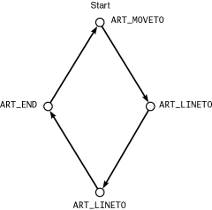
Each element consists of a single coordinate point and one property, the ArtPathcode enumeration, which tells libart how this point connects to the previous point, if any:
typedef enum
{
  ART_MOVETO,
  ART_MOVETO_OPEN,
  ART_CURVETO,
  ART_LINETO,
  ART_END
} ArtPathcode;
|
The first point in a path array must be ART_MOVETO if the path is a closed path or ART_MOVETO_OPEN for an open path. The final point is always ART_END. All other points in a vector path array must be ART_LINETO. In a closed path, libart will implicitly connect the ART_END point to the initial ART_MOVETO point.
By definition, a vector path consists of all straight lines. For this reason, ART_CURVETO is not permitted in vector paths. As we will see in the next section, the more complex Bezier paths can handle curves.
Bezier Paths
When you can get away with only straight lines, use vector paths. The calculations are simple and fast, and the paths are easy to build. However, if you are trying to draw anything natural-looking, straight lines will make it look blocky and clumsy. At some point you will probably want to render a real curve. This is where Bezier paths come into play.
Each element of a Bezier path requires three coordinate points rather than the single point used by a vector path element. In a nutshell, the Bezier curve is defined by its starting and ending points, as well as a middle point, usually off to the side. The curve will trace a path from the first coordinate to the final coordinate, pulled away from a straight line by the middle coordinate in a pre- dictable, mathematical curve. This path is defined by the following cubic equations, where t goes from 0 to 1:
x = x0(1 - t)3 + x1(1 - t)2t + x2(1 - t)t2 + x3t3
y = y0(1 - t)3 + y1(1 - t)2t + y2(1 - t)t2 + y3t3
|
Libart uses the following data structure to hold the data for each Bezier line segment; a Bezier path is an array of one or more of these segments. It can be open or closed, and it can be a mixture of straight lines (where only the x3 and y3 coordinates are used) and curved lines.
typedef struct _ArtBpath ArtBpath;
struct _ArtBpath
{
  ArtPathcode code;
  double x1;
  double y1;
  double x2;
  double y2;
  double x3;
  double y3;
};
|
Sorted Vector Paths
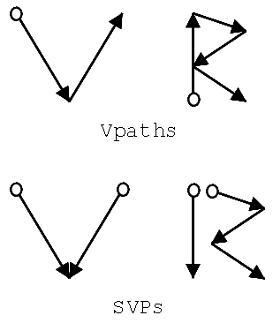
As part of its suite of optimizations, libart defines a sorted vector path (SVP) to organize a normal vector path into groups of similar segments. Each SVP element consists of two or more points (i.e., a vector path) tracing a path of coordinates that steadily increases or decreases along the y-axis. This rule helps optimize algorithms that render in a vertical direction, in particular those used to display image buffers on the screen.
Consider a path shaped like the letter V. A vector path would describe it with a downward (increasing y-axis) stroke, followed by an upward (decreasing y-axis) stroke. A sorted vector path would break it up into two downward strokes converging on the same point, thus making it easier to render the V from the top down. Figure 10.6 shows the letters V and R broken down into vector paths and sorted vector paths.
Another important feature of SVPs that helps optimize their rendering code is the bounding box assigned to each SVP segment. This bounding box defines the minimum rectangular area that can contain that SVP segment (which, remember, can contain more than two points, like the second segment in the "R" example). When part or all of a sorted vector path needs to be redrawn, the area that must be "dirtied" can be clipped and reduced quite a bit, so that only the areas covered by those bounding boxes are repainted rather than a single, huge rectangle that covers the entire path. This clipping can save a lot of needless work.
Microtile Arrays
Libart's microtile arrays make it easier to optimize image redrawing, by breaking the "dirty" areas down into smaller rectangles. The microtile array (affectionately abbreviated uta, with the "u" standing for the Greek letter m, or micron) represents a grid of 32 32 pixel squares overlaid on an area of coordinate space. For example, a 96 64 pixel buffer would have six microtiles, arranged in a 3 2 grid.
Figure 10.7 shows a path drawn in the shape of a guitar case. Rather than having to rerender the bounding box of the entire path, indicated by the dotted line, the microtile array breaks the dirty regions into smaller components. The gray rectangles show the areas that need to be refreshed when using the uta.
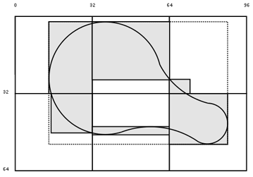
Each microtile has a single bounding box within its 32 32 area, to mark the entire area of interest-the "dirty" area in the case of repainting algorithms-within its grid square. When an application attempts to refresh its microtiled drawing areas, it can roll through the uta and redraw only the area contents of each bounding box. It can ignore all microtiles with zero-area bounding boxes. The fewer unnecessary pixels the application has to redraw, the faster the refresh will take place each time. In practice, the microtiles are usually merged and decomposed into an array of rectangles, optimized for efficient redraws.
A significant advantage to utas is that you can add to them dynamically, as the dirty area changes. The microtiles will adjust their bounding boxes to include the new areas or ignore the areas they already cover. This makes it much easier to implement deferred painting updates, in which redraws happen during idle times. Between updates, the microtiles accumulate "dirt," but they always remain in a ready-to-use state, whenever the next repaint event happens to occur.
Another advantage of microtile arrays is their stable memory footprint. No matter how many times a drawing area is damaged, the number of microtiles never increases. Only the coordinates of the existing bounding boxes change. Utas are also very efficient, especially because of their 32-pixel grid size. The 32-pixel boundaries result in convenient 4-byte-aligned chunks of the pixel buffer. Also, the fact that each bounding box is constrained to a coordinate range of 0 to 32 pixels makes it possible to fit all four coordinate values into a single 32-bit integer. Technically, each coordinate fits into 5 bits, but to maintain the optimization, each coordinate is padded to 8 bits. Thus our earlier 96 64 pixel example requires only 24 bytes (6 microtiles 4 bytes) to express its bounding-box data.
Affine Transformations
Now that we have the basic building blocks of a vector drawing kit, we need some way to move those vectors around. At the very least, we should be able to move them through space, or translate them. Another important feature is scaling them to larger or smaller sizes, to simulate zooming and unzooming. Even more sophisticated is the ability to rotate our lines and polygons. Finally, we might like to be able to shear our vector paths-for example, to turn a normal rectangle into a slanted parallelogram.
Libart implements these operations as affine transforms; each transform is characterized by an array-or matrix-of six floating-point numbers. To apply the affine transform on a path, libart passes each coordinate pair through these two operations, where x and y are the old coordinates, x' and y' are the new coordinates, and affine0 through affine5 make up the array of floating-point numbers:
x' = affine0x + affine2y + affine4
y' = affine1x + affine3y + affine5
|
Surprisingly, these innocent-appearing little functions can result in quite a number of dazzling effects, in particular the four transforms already mentioned. By carefully tweaking the affine matrix, we can invent many strange new transforms. Of particular note is the simplicity of the calculations. Affine transforms involve only multiplication and addition, two fairly quick operations that are not likely to bog down your rendering routines. You don't have to worry about any complicated square roots or cubic equations sneaking into your back-end algorithms.
The simplest transform of all is identity, which leaves all points in the path unaltered. The identity looks like (1, 0, 0, 1, 0, 0) and simplifies to the following equations:
x' = 1x + 0y + 0 = x
y' = 0x + 1y + 0 = y
|
A translation transform is a simple offset, which looks like (1, 0, 0, 1, m, n), in which every point is moved m units horizontally and n units vertically:
x' = 1x + 0y + m = x + m
y' = 0x + 1y + n = y + n
|
Scaling is similar to the identity transform, except it uses values greater or less than 1 and looks like (m, 0, 0, n, 0, 0). Values greater than 1 will enlarge, or zoom in, and values between 0 and 1 will shrink, or zoom out. Negative values will flip the path to the opposite side of the axis, which is not normally what you want, so you'll probably want to keep your multipliers in the positive range:
x' = mx + 0y + 0 = mx
y' = Ox + ny + 0 = ny
|
Rotation and shearing transforms are a little more complex, and they usually involve some sort of trigonometry. To see how they work, take a look at libart's implementation of them. The source code is in the gnome-libs package in the file gnome-libs/libart_lgpl/art_affine.c, located in the art_affine_rotate( ) and art_affine_shear( ) functions. The other mentioned transforms reside in art_affine_identity( ), art_affine_translate( ), and art_affine_scale( ). You'll find other interesting transforms in art_affine_invert( ), art_affine_flip( ), and art_affine_point( ); you can compare two transforms with art_affine_equal( ) and combine two transforms with art_affine_multiply( ). If you use only one thing in libart, it will most likely be the affine transforms, so it's a good idea to figure out how they work. They also pop up from time to time in the GNOME Canvas (see Chapter 11).
Affine transformations have some very interesting properties that make their simplicity even more attractive. First, affines are linear, so they always transform straight lines into straight lines; also, if two lines are parallel, they will remain parallel after any number of transforms. Closed paths will remain closed.
Another interesting property is that affine transforms are cumulative. You can combine multiple transforms into a single composite transform with art_affine_multiply( ), so if you have a series of transformations that you always perform in order, you can speed things up by combining them into a single transform. The results will be exactly the same. Note, however, that order is still important. If you exchange steps 3 and 4 in a six-step series, you will very likely come out with different results (depending on the specifics of the transforms; obviously if steps 3 and 4 were both identity transforms, it wouldn't matter).
Finally, affine transforms are mathematically reversible. You can apply a transform, invert it with art_affine_invert( ), and apply the inversion, and you will end up with your original path (taking into account any rounding errors).
Pixel Buffers
One of the highlights of libart is its support for RGB and RGBA (red-green-blue-alpha) pixel buffers, or pixbufs. All of the various data constructs and algorithms come to fruition in these buffers. You can draw lines and shapes on the pixel buffer by creating an SVP (or by creating a vector path and converting that into an SVP) and rendering it to the pixbuf with a stroking operation. You can apply any number of affine transforms on images to offset, scale, and otherwise morph them. Libart also provides pixel buffer life cycle management in the form of creation and destruction functions.
Libart defines its own data structure, ArtPixBuf, to hold the important elements:
typedef struct _ArtPixBuf ArtPixBuf;
struct _ArtPixBuf
{
  ArtPixFormat format;
  int n_channels;
  int has_alpha;
  int bits_per_sample;

  art_u8 *pixels;
  int width;
  int height;
  int rowstride;
  void *destroy_data;
  ArtDestroyNotify destroy;
};
|
Most of the fields in ArtPixBuf should look familiar from our discussions in the earlier parts of this chapter. Only a few of them represent new concepts.
The format field holds the structural format of the pixel buffer. For now, the ArtPixFormat enumeration allows only one value, ART_PIX_RGB, signifying a three-or four-channel RGB buffer. In the future, libart might support other color formats, such as grayscale, CMYK (cyan-magenta-yellow-black), and so on.
The n_channels field determines the number of color channels the pixel buffer has. A three-color RGB buffer has three channels; a three-color RGB pixel buffer with an alpha channel has an n_channels of 4. All other values are invalid for ART_PIX_RGB.
ArtPixBuf explicitly states whether or not one of its channels is an alpha channel with the has_alpha field. Although you can probably figure this out by looking at n_channels, you should avoid doing so. Other pixbuf formats may have a different number of base channels. For example, grayscale might have one color channel and one alpha channel, while CMYK might have four color channels and one alpha channel. The has_alpha field is the only surefire way to test for the presence of an alpha channel.
The bits_per_sample field is another way of expressing the color depth of the pixel buffer. A sample is analogous to a color channel, so we can calculate the bit depth of a buffer by multiplying n_channels by bits_per_sample. Normally this value stays at 8, implying 24-bit color depth for a three-channel RGB pixbuf.
The next four fields describe the structure of the buffer. The pixels field points to the actual buffer data, which is simply an array of unsigned char (defined by typedef to art_u8). The width, height, and rowstride fields control how the pixels array is divided into rows and columns, with potential padding bytes at the end of each row, as indicated by rowstride.
The final two fields, destroy_data and destroy, are optional fields that permit you to register a callback function that libart will invoke just before it destroys the ArtPixBuf instance. You don't need to register the destroy callback unless you have data of your own that you'd like automatically cleaned up when the owning ArtPixBuf instance is destroyed. The ArtDestroyNotify function prototype looks like this:
typedef void (*ArtDestroyNotify) (void *func_data, void *data);
|
Libart provides several functions to automatically fill in these fields with the proper values. You use a different function to create a three-channel pixel buffer than you do to create a four-channel buffer, and yet another set of functions if you want to register a destroy callback. Here's a quick listing of the commonly used ArtPixBuf creation and destruction functions:
ArtPixBuf* art_pixbuf_new_rgb(art_u8 *pixels,
    int width, int height, int rowstride);
ArtPixBuf* art_pixbuf_new_rgba(art_u8 *pixels,
    int width, int height, int rowstride);
ArtPixBuf* art_pixbuf_new_rgb_dnotify(art_u8 *pixels,
    int width, int height, int rowstride,
    void *dfunc_data, ArtDestroyNotify dfunc);
ArtPixBuf* art_pixbuf_new_rgba_dnotify(art_u8 *pixels,
    int width, int height, int rowstride,
    void *dfunc_data, ArtDestroyNotify dfunc);
void art_pixbuf_free (ArtPixBuf *pixbuf);
|
You may have noticed that ArtPixBuf has a lot of fields similar to those found in the GdkRGB API. It even seems to implement a fair amount of the same functionality. Although at first this may seem like a duplication of effort,2 the two APIs are kept separate for good reason. GdkRGB is intimately tied to GDK, and by extension to GLib. Most of GdkRGB's focus is on rendering pixel buffers to GDK drawables, performing dithering, and managing color maps-all operations that are very specific to windowing systems.
On the other hand, libart is very generic, with as few external dependencies as possible. For this reason libart can survive outside of GTK+ and GNOME; it doesn't even need GLib. Libart is free from all windowing-system and GUI constraints. In the true UNIX spirit, it does one thing and it does it very well: pixel buffer manipulation. Thus if you want to make use of libart, you will have to provide your own code to transfer the contents of the ArtPixBuf structures to a drawing widget of some sort. Usually the easiest way is to transfer your pixel buffers to a G+kDrawingArea widget, using GdkRGB. The GNOME Canvas implements a similar approach in its anti-aliased mode, using GdkRGB and the Canvas widget (see Chapter 11).