 |
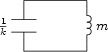
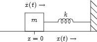
Consider now the mass-spring oscillator depicted physically in Fig.B.3, and in equivalent-circuit form in Fig.B.4.
|
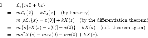
By Newton's second law of motion, the force ![]() applied to a mass
equals its mass times its acceleration:
applied to a mass
equals its mass times its acceleration:
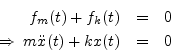
We have thus derived a second-order differential equation governing
the motion of the mass and spring. (Note that ![]() in
Fig.B.3 is both the position of the mass and compression
of the spring at time
in
Fig.B.3 is both the position of the mass and compression
of the spring at time ![]() .)
.)
Taking the Laplace transform of both sides of this differential equation gives
To simplify notation, denote the initial position and velocity by
![]() and
and
![]() , respectively. Solving for
, respectively. Solving for ![]() gives
gives
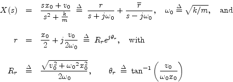
denoting the modulus and angle of the pole residue ![]() , respectively.
From §B.1, the inverse Laplace transform of
, respectively.
From §B.1, the inverse Laplace transform of ![]() is
is
![]() , where
, where ![]() is the Heaviside unit step function at time 0.
Then by linearity, the solution for
the motion of the mass is
is the Heaviside unit step function at time 0.
Then by linearity, the solution for
the motion of the mass is
![\begin{eqnarray*}
x(t) &=& re^{-j{\omega_0}t} + \overline{r}e^{j{\omega_0}t}
= ...
...ga_0}t - \tan^{-1}\left(\frac{v_0}{{\omega_0}x_0}\right)\right].
\end{eqnarray*}](img1699.png)
If the initial velocity is zero (![]() ), the above formula
reduces to
), the above formula
reduces to
![]() and the mass simply oscillates sinusoidally at frequency
and the mass simply oscillates sinusoidally at frequency
![]() , starting from its initial position
, starting from its initial position ![]() .
If instead the initial position is
.
If instead the initial position is ![]() , we obtain
, we obtain