When the state transition matrix ![]() is diagonal, we have the
so-called modal representation. In the single-input,
single-output (SISO) case, the general diagonal system looks like
is diagonal, we have the
so-called modal representation. In the single-input,
single-output (SISO) case, the general diagonal system looks like
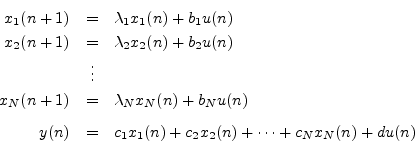
Thus, the diagonalized state-space system consists of ![]() parallel one-pole systems. See §9.2.2
and §6.8.7 regarding the conversion of direct-form filter
transfer functions to parallel (complex) one-pole form.
parallel one-pole systems. See §9.2.2
and §6.8.7 regarding the conversion of direct-form filter
transfer functions to parallel (complex) one-pole form.
![$\displaystyle \left[\begin{array}{c} x_1(n+1) \\ [2pt] x_2(n+1) \\ [2pt] \vdots \\ [2pt] x_{N-1}(n+1)\\ [2pt] x_N(n+1)\end{array}\right]$](img2112.png)
![\begin{displaymath}\left[
\begin{array}{ccccc}
\lambda _1 & 0 & 0 & \cdots & 0 \...
...ts \\ [2pt] b_{N-1}\\ [2pt] b_N\end{array}\right] u(n)\nonumber\end{displaymath}](img2114.png)