Input
Signal 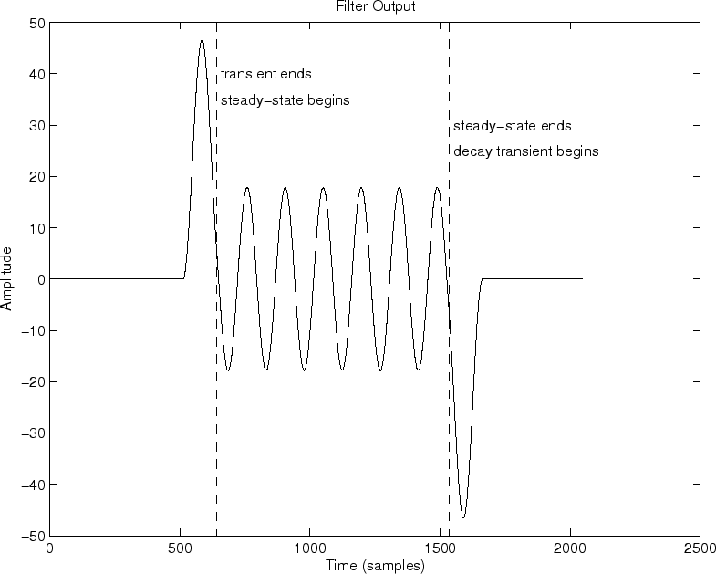
Filter Output Signal
|
|
Input
Signal
Filter Output Signal
|
The terms transient response and steady state response arise naturally in the context of sinewave analysis (e.g., §2.2). When the input sinewave is switched on, the filter takes a while to ``settled down'' to a perfect sinewave at the same frequency, as illustrated in Fig.5.7(b). The filter response during this ``settling'' period is called the transient response of the filter. The response of the filter after the transient response, provided the filter is linear and time-invariant, is called the steady-state response, and it consists of a pure sinewave at the same frequency as the input sinewave, but with amplitude and phase determined by the filter's frequency response at that frequency. In other words, the steady-state response begins when the LTI filter is fully ``warmed up'' by the input signal. More precisely, the filter output is the same as if the input signal had been applied since time minus infinity.
For length ![]() FIR filters, the duration of the transient response is
FIR filters, the duration of the transient response is
![]() samples. To make this clear, consider that a length
samples. To make this clear, consider that a length ![]() (zero-order) FIR filter (a simple gain), has no state memory at all,
and thus it is in ``steady state'' immediately when the input signal
is switched on because it has one sample of memory for storing the
previous input sample. A length
(zero-order) FIR filter (a simple gain), has no state memory at all,
and thus it is in ``steady state'' immediately when the input signal
is switched on because it has one sample of memory for storing the
previous input sample. A length ![]() FIR filter, on the other hand,
reaches steady state one sample after the input sinewave is switched
on. At the switch-on time instant, the length 2 FIR filter has a
single sample of state that is still zero instead of the previous
input sinewave sample. In general, a length
FIR filter, on the other hand,
reaches steady state one sample after the input sinewave is switched
on. At the switch-on time instant, the length 2 FIR filter has a
single sample of state that is still zero instead of the previous
input sinewave sample. In general, a length ![]() FIR filter is fully
``warmed up'' after the input sample at time
FIR filter is fully
``warmed up'' after the input sample at time ![]() ; that is, for an
input starting at time
; that is, for an
input starting at time ![]() , by time
, by time ![]() , all internal state
delays of the filter contain delayed input samples instead of their
initial zeros.
, all internal state
delays of the filter contain delayed input samples instead of their
initial zeros.
The signals for the plots above were computed as follows:
N = 1024; % input signal length (nonzero portion)
Nh = N/8; % FIR filter length
A = 1; B = ones(1,Nh); % FIR "moving average" filter
n = 0:N-1;
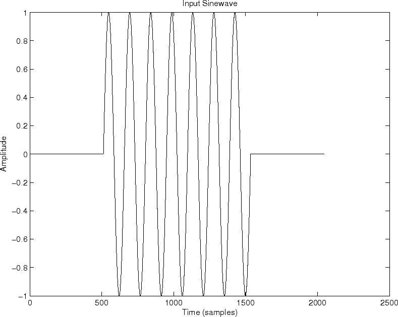
x = sin(n*2*pi*7/N); % input sinusoid - zero-pad it:
zp=zeros(1,N/2); xzp=[zp,x,zp]; nzp=[0:length(xzp)-1];
y = filter(B,A,xzp); % filtered output signal
The input signal is plotted in Fig.5.7(a), and the
corresponding output signal is plotted in Fig.5.7(b). We can
now see that the transient response must end
Since the coefficients of an FIR filter are also its nonzero impulse response samples, we can say that the duration of the transient response equals the length of the impulse response minus one.
For Infinite Impulse Response (IIR) filters, such as the recursive
comb filter analyzed in Chapter 3, the transient response
decays exponentially. This means it is never really completely
finished. In other terms, since its impulse response is infinitely
long, so is its transient response, in principle. However, in
practice, we treat it as finished for all practical purposes after
several time constants of decay. For example, seven time-constants of
decay correspond to more than 60 dB of decay, and is a common cut-off
used for audio purposes. Therefore, we can adopt ![]() as the
definition of decay time (or ``ring time'') for typical
audio filters. See [83]6.5 for a detailed derivation of
as the
definition of decay time (or ``ring time'') for typical
audio filters. See [83]6.5 for a detailed derivation of
![]() and related topics. In summary, we can say that the
transient response of an audio filter is over after
and related topics. In summary, we can say that the
transient response of an audio filter is over after ![]() seconds,
where
seconds,
where ![]() is the time it takes the filter impulse response to
decay by
is the time it takes the filter impulse response to
decay by ![]() dB.
dB.
Figure 5.8 plots an IIR filter example for the filter
![]() . The previous matlab is modified as follows:
. The previous matlab is modified as follows:
      B = 1; A = [1 -0.99];
      Nh = 300; % APPROXIMATE filter length (visually in plot)
      B = 1; A = [1 -0.99]; % One-pole recursive example
      ...       % otherwise as above for the FIR example
The decay time for this recursive filter was arbitrarily marked at 300
samples (about three time-constants of decay).

Input
Signal 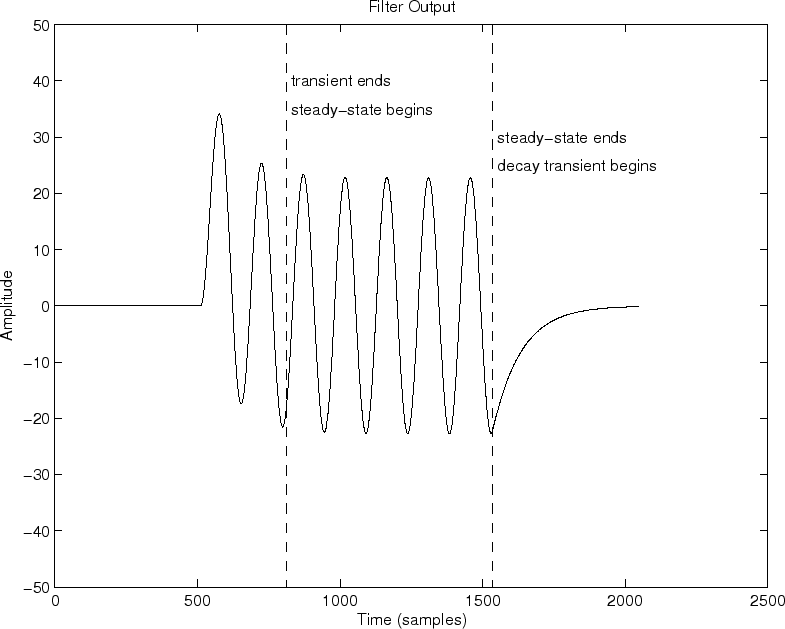
Filter Output Signal
|