The difference equation is a formula for computing an output
sample at time ![]() based on past and present input samples and past
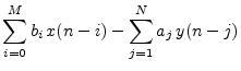
output samples in the time domain.6.1We may write the general, causal, LTI difference equation as follows:
based on past and present input samples and past
output samples in the time domain.6.1We may write the general, causal, LTI difference equation as follows:
As a specific example, the difference equation
When the coefficients are real numbers, as in the above example, the filter is said to be real. Otherwise, it may be complex.
Notice that a filter of the form of Eq. (5.1) can use ``past''
output samples (such as ![]() ) in the calculation of the
``present'' output
) in the calculation of the
``present'' output ![]() . This use of past output samples is called
feedback. Any filter having one or more
feedback paths (
. This use of past output samples is called
feedback. Any filter having one or more
feedback paths (![]() ) is called
recursive. (By
the way, the minus signs for the feedback in Eq. (5.1) will be
explained when we get to transfer functions in §6.1.)
) is called
recursive. (By
the way, the minus signs for the feedback in Eq. (5.1) will be
explained when we get to transfer functions in §6.1.)
More specifically, the ![]() coefficients are called the
feedforward coefficients and the
coefficients are called the
feedforward coefficients and the ![]() coefficients are called
the feedback coefficients.
coefficients are called
the feedback coefficients.
A filter is said to be recursive if and only if ![]() for
some
for
some ![]() . Recursive filters are also called
infinite-impulse-response (IIR) filters.
When there is no feedback (
. Recursive filters are also called
infinite-impulse-response (IIR) filters.
When there is no feedback (
![]() ), the filter is said
to be a nonrecursive or
finite-impulse-response (FIR) digital filter.
), the filter is said
to be a nonrecursive or
finite-impulse-response (FIR) digital filter.
When used for discrete-time physical modeling, the difference equation may be referred to as an explicit finite difference scheme.6.2
Showing that a recursive filter is LTI (Chapter 4) is easy by considering its impulse-response representation (discussed in §5.6). For example, the recursive filter
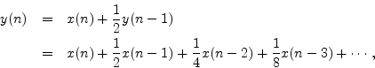
has impulse response
![]() ,
,
![]() . Since
the impulse response is the same no matter when the impulse occurs
(time invariant), and since the impulse response values do not depend
on the input amplitude (linear), the filter is LTI.
. Since
the impulse response is the same no matter when the impulse occurs
(time invariant), and since the impulse response values do not depend
on the input amplitude (linear), the filter is LTI.