 |
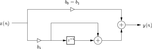
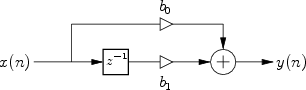
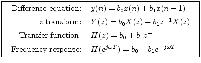
Figure 10.1 gives the signal flow graph for the general one-zero filter. The frequency response for the one-zero filter may be found by the following steps:
By factoring out
![]() from the frequency response, to
balance the exponents of
from the frequency response, to
balance the exponents of ![]() , we can get this closer to polar form as
follows:
, we can get this closer to polar form as
follows:
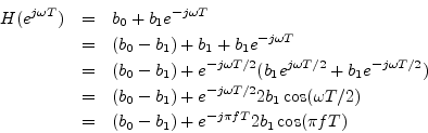
This is the frequency response of the filter in Fig.10.1.
 |
The term ![]() may be interpreted as an order 0 filter section
(``volume knob'') with gain
may be interpreted as an order 0 filter section
(``volume knob'') with gain
![]() . This gain control is in
parallel (i.e., summed) with a first-order section
. This gain control is in
parallel (i.e., summed) with a first-order section
![]() having an amplitude response that varies sinusoidally from 2 to 0 as
frequency goes from 0 to half the sampling rate (which is
the behavior of our simplest lowpass filter example analyzed in Chapter 1).
Figure 10.2 illustrates this interpretation of the general
one-zero filter. Thus, the general one-zero filter can be interpreted
as a digital volume knob in parallel with the series combination of
another gain control and the simplest lowpass filter.
having an amplitude response that varies sinusoidally from 2 to 0 as
frequency goes from 0 to half the sampling rate (which is
the behavior of our simplest lowpass filter example analyzed in Chapter 1).
Figure 10.2 illustrates this interpretation of the general
one-zero filter. Thus, the general one-zero filter can be interpreted
as a digital volume knob in parallel with the series combination of
another gain control and the simplest lowpass filter.
Representing the general one-zero filter as a volume control in
parallel with a scaled two-point average is useful for visualizing the
possible range of frequency responses. For completeness, however, we
now apply the general equations given in
Chapter 7 for filter gain ![]() and filter phase
and filter phase
![]() as a function of frequency:
as a function of frequency:
![\begin{eqnarray*}
H(e^{j\omega T}) &=& b_0 + b_1e^{-j\omega T}\\
&=& b_0 + b_1...
...left[\frac{-b_1 \sin(\omega T)}{b_0 + b_1 \cos(\omega T)}\right]
\end{eqnarray*}](img1214.png)
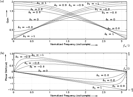
A plot of ![]() and
and
![]() for
for ![]() and various
values of
and various
values of ![]() , is given in Fig.10.3. The filter has a zero
at
, is given in Fig.10.3. The filter has a zero
at
![]() in the
in the ![]() plane, which is always on the
real axis. When a point on the unit circle comes close to the zero of
the transfer function the filter gain at that frequency is
low. Notice that one real zero can basically make either a highpass
(
plane, which is always on the
real axis. When a point on the unit circle comes close to the zero of
the transfer function the filter gain at that frequency is
low. Notice that one real zero can basically make either a highpass
(
![]() ) or a lowpass filter (
) or a lowpass filter (
![]() ). For the phase
response calculation using the graphical method, it is necessary to
include the pole at
). For the phase
response calculation using the graphical method, it is necessary to
include the pole at ![]() .
.