Group Delays
|
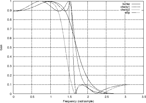
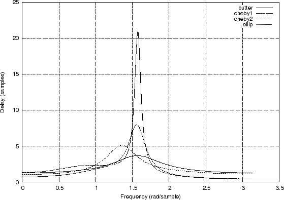
Figure 7.6 compares the group delay responses for a number of classic lowpass filters, including the example of Fig.7.2. The matlab code is listed in Fig.7.5. See, e.g., Parks and Burrus [63] for a discussion of Butterworth, Chebyshev, and Elliptic Function digital filter design. See also §G.2 for details on the Butterworth case. The various types may be summarized as follows:
As Fig.7.6(b) indicates, and as is well known, the Butterworth filter has the flattest group delay curve (and most gentle transition from passband to stopband) for the four types compared. The elliptic function filter has the largest amount of ``delay distortion'' near the cut-off frequency (passband edge frequency). Fundamentally, the more abrupt the transition from passband to stopband, the greater the delay-distortion across that transition, for any minimum-phase filter. (Minimum-phase filters are introduced in Chapter 12). The delay-distortion can be compensated by delay equalization, i.e., adding delay at other frequencies in order approach an overall constant group delay versus frequency. Delay equalization is typically carried out using an allpass filter in series with the filter to be delay-equalized [1]. (Allpass filters are discussed in §10.2.)
[Bb,Ab] = butter(4,0.5); % order 4, cutoff at 0.5 * pi Hb=freqz(Bb,Ab); Db=grpdelay(Bb,Ab); [Bc1,Ac1] = cheby1(4,1,0.5); % 1 dB passband ripple Hc1=freqz(Bc1,Ac1); Dc1=grpdelay(Bc1,Ac1); [Bc2,Ac2] = cheby2(4,20,0.5); % 20 dB stopband attenuation Hc2=freqz(Bc2,Ac2); Dc2=grpdelay(Bc2,Ac2); [Be,Ae] = ellip(4,1,20,0.5); % like cheby1 + cheby2 He=freqz(Be,Ae); [De,w]=grpdelay(Be,Ae); figure(1); plot(w,abs([Hb,Hc1,Hc2,He])); grid('on'); xlabel('Frequency (rad/sample)'); ylabel('Gain'); legend('butter','cheby1','cheby2','ellip'); saveplot('../eps/grpdelaydemo1.eps'); figure(2); plot(w,[Db,Dc1,Dc2,De]); grid('on'); xlabel('Frequency (rad/sample)'); ylabel('Delay (samples)'); legend('butter','cheby1','cheby2','ellip'); saveplot('../eps/grpdelaydemo2.eps'); |
|
Group Delays
|