Phase Unwrapping

In working with phase delay, it is often necessary to ``unwrap'' the phase response $\Theta(\omega)$. Phase unwrapping ensures that all appropriate multiples of $2\pi$ have been included in $\Theta(\omega)$. We defined $\Theta(\omega)$ simply as the complex angle of the frequency response $H(e^{j\omega T})$, and this is not sufficient for obtaining a phase response which can be converted to true time delay. If multiples of $2\pi$ are discarded, as is done in the definition of complex angle, the phase delay is modified by multiples of the sinusoidal period. Since LTI filter analysis is based on sinusoids without beginning or end, one cannot in principle distinguish between ``true'' phase delay and a phase delay with discarded sinusoidal periods when looking at a sinusoidal output at any given frequency. Nevertheless, it is often useful to define the filter phase response as a continuous function of frequency with the property that $\Theta(0) = 0$ or $\pi$ (for real filters). This specifies how to unwrap the phase response at all frequencies where the amplitude response is finite and nonzero. When the amplitude response goes to zero or infinity at some frequency, we can try to take a limit from below and above that frequency.

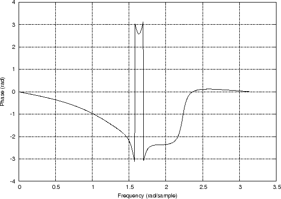
Matlab and Octave have a function called unwrap() which implements a numerical algorithm for phase unwrapping. Figures 7.4(a) and 7.4(b) show the effect of the unwrap function on the phase response of the example elliptic lowpass filter of §7.5.2, modified to contract the zeros from the unit circle to a circle of radius $0.95$ in the $z$ plane:

  [B,A] = ellip(4,1,20,0.5); % design lowpass filter
   B = B .* (0.95).^[1:length(B)]; % contract zeros by 0.95
  [H,w] = freqz(B,A);      % frequency response
  theta = angle(H);        % phase response
  thetauw = unwrap(theta); % unwrapped phase response

In Fig.7.4(a), the phase-response minimum has ``wrapped around'' to the top of the plot. In Fig.7.4(b), the phase response is continuous. We have contracted the zeros away from the unit circle in this example, because the phase response really does switch discontinuously by $\pi$ radians when frequency passes through a point where the phases crosses zero along the unit circle (see Fig.7.3(b)). The unwrap function need not modify these discontinuities, but it is free to add or subtract any integer multiple of $2\pi$ in order to obtain the ``best looking'' discontinuity. Typically, for best results, such discontinuities should alternate between $+\pi$ and $-\pi$, making the phase response resemble a distorted ``square wave'', as in Fig.7.3(b). A more precise example appears in Fig.11.2.

Figure 7.4: Phase response of a modified order 4 elliptic function lowpass filter cutting off at $f_s/4$.

Phase Response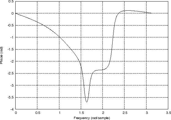

Unwrapped Response